Credit Supply and the Rise in College Tuition: Evidence from the

This paper presents preliminary findings and is being distributed to economists

and other interested readers solely to stimulate discussion and elicit comments.

The views expressed in this paper are those of the authors and do not necessarily

reflect the position of the Federal Reserve Bank of New York or the Federal

Reserve System. Any errors or omissions are the responsibility of the authors.

Federal Reserve Bank of New York

Staff Reports

Credit Supply and the Rise in College

Tuition: Evidence from the Expansion in

Federal Student Aid Programs

David O. Lucca

Taylor Nadauld

Karen Shen

Staff Report No. 733

July 2015

Revised February 2017

Credit Supply and the Rise in College Tuition: Evidence from the Expansion in Federal

Student Aid Programs

David O. Lucca, Taylor Nadauld, and Karen Shen

Federal Reserve Bank of New York Staff Reports, no. 733

July 2015; revised February 2017

JEL classification: G28, I22

Abstract

We study the link between the student credit expansion of the past fifteen years and the

contemporaneous rise in college tuition. To disentangle simultaneity issues, we analyze the

effects of increases in federal student loan caps using detailed student-level financial data. We

find a pass-through effect on tuition of changes in subsidized loan maximums of about 60 cents

on the dollar, and smaller but positive effects for unsubsidized federal loans. The subsidized loan

effect is most pronounced for more expensive degrees, those offered by private institutions, and

for two-year or vocational programs.

Key words: student loans, college tuition

_________________

Lucca: Federal Reserve Bank of New York (e-mail: david.lucca@ny.frb.org). Nadauld: Brigham

Young University (e-mail: taylor.nadauld@byu.edu). Shen: Harvard University (e-mail:

[email protected]ard.edu). The authors thank Brian Melzer (discussant), Ian Fillmore, Paul

Goldsmith-Pinkham, Erik Hurst, Lance Lochner, Christopher Palmer (discussant), Johannes

Stroebel (discussant), Sarah Turner, and seminar participants at the American Finance

Association’s 2016 annual meeting, the Federal Reserve Bank of New York, Brigham Young

University, the NBER 2015 SI Corporate Finance Workshop, and the Julis-Rabinowitz Center

for Public Policy and Finance’s Annual Conference for helpful comments and discussions. The

authors also thank Carter Davis for providing excellent research assistance. The views expressed

in this paper are those of the authors and do not necessarily reflect the position of the Federal

Reserve Bank of New York or the Federal Reserve System.

1 Introduction

The existence of a causal link between student loan availability and college tuition has been

the subject of policy discussion and debate for at least three decades (Bennett, 1987, for example),

and has been no less relevant in recent years as tuition and student loan balances have continued

to signiﬁcantly outpace overall inﬂation. Average sticker-price tuition rose 46% in constant 2012

dollars between 2001 and 2012 (Figure 1), and despite a sharp deleveraging of other sources of

debt by U.S. households after the Great Recession, student debt has continued to grow unabated,

and now represents the largest form of non-mortgage liability for households (Figure 2). While

rising tuition almost certainly contributes to increased demand for student loans, an important

policy question is whether student loan supply may also allow tuition to rise as postulated by the

so-called “Bennett Hypothesis.”

In this paper, we propose an identiﬁcation strategy to isolate the eﬀect of student loans on

tuition. We use variation in student credit supply that resulted from legislative changes in the

maximum amounts students are eligible to borrow from the federal subsidized and unsubsidized

loan programs. These policy changes went into eﬀect in the 2007-08 and 2008-09 school years and

led to a large credit expansion, as these program maximums had remained unchanged since the

early 1990s.

Exploiting the federal increase in credit supply for identiﬁcation presents two chal-

lenges. First, the increase in program maximums aﬀected students at all institutions. Second, we

only have reliable time series data on the sticker-price of tuition rather than the net tuition paid by

students after accounting for scholarships or discounts to lower-income students. In an illustra-

tive model, however, we show that even when universities price-discriminate, a credit expansion

will raise tuition paid by all students, not just students borrowing at the federal loan caps, because

of pecuniary demand externalities. We also show that the tuition eﬀects will be larger at schools

The then-Secretary of Education William Bennett (1987) argued that “[...] increases in ﬁnancial aid in recent years

have enabled colleges and universities blithely to raise their tuitions, conﬁdent that Federal loan subsidies would help

cushion the increase,” a statement that came to be known as the “Bennett Hypothesis.”

The maximum subsidized federal loan amount for freshmen rose in the 2007-08 academic year from $2,625 to $3,500,

and for sophomores from $3,500 to $4,500; unsubsidized loan maximums rose by $2,000 in the academic year 2008-09.

Pell Grant maximums, which is not our main focus but that we control for, rose gradually between the 2007-2008 and

2010-2011 school years as well as in prior years as a result of the yearly appropriation process of the Department of Ed-

ucation. Subsidized, unsubsidized loans and Pell Grants are the main “Title IV” programs. We discuss the institutional

details of federal aid programs in Section 3.

serving a more credit-constrained population. We use these predictions to identify the impact of

loan supply increases on tuition by constructing an institution’s “exposure,” or treatment intensity,

to a policy change using detailed student-level data. We then interact our exposure measure with

the timing of shifts in the supply of federal student aid, with an approach similar to Card (1999)’s

analysis of changes in national minimum wage standards.

We ﬁrst validate our approach by documenting that institution-level loan amounts respond

to the interaction of the legislated changes in maximum aid amounts with an institution’s expo-

sure to the changes. Changes in per-student subsidized (unsubsidized) loan amounts measured

at the institution level load with a coeﬃcient of .7 (.6) on yearly changes in the maximums per

qualifying student. We next study the response of tuition to the interaction of policy changes and

treatment intensity to examine tuition increases in the same year as the credit expansions. We ﬁnd

that increases in institution-speciﬁc subsidized (unsubsidized) loan maximums lead to a sticker-

price increase of about 60 (40) cents on the dollar. This eﬀect represents the additional amount that

institutions raised their tuition in the years of the policy changes relative to what would have been

expected without the policy change, which we measure using institutional ﬁxed eﬀects to capture

the average tuition increases at an institution. All of these eﬀects are highly signiﬁcant and con-

sistent with the Bennett Hypothesis, and apply to a large sample of all Title IV institutions. Direct

quotes from earnings calls and large stock market reactions to the passing of these loan expansions

lend additional support to these ﬁndings for the subset of publicly traded for-proﬁt institutions.

The eﬀect that we document is particularly interesting because it is evidence of a cross-demand

eﬀect of a credit expansion through a pecuniary externality with a relaxation of the borrowing con-

straint for some students aﬀecting pricing to other students. Of course, institutions may have miti-

gated the eﬀect of these increases through increases in institutional grants to some or all students.

Though institutional grant data is not available for our entire sample, we ﬁnd that an increase in

subsidized loans actually decreased institutional grants by about 20 cents on the dollar (compared

to an eﬀect of about 30 cents for Pell Grants) for the subset of institutions that report grant amounts,

suggesting that the tuition eﬀect is on average not canceled out, and may even be ampliﬁed, by in-

stitutional grants, though we cannot observe the distribution of grants.

In robustness checks and alternative speciﬁcations, we attempt to address concerns that other

variables may be driving the behavior we observe. First of all, our speciﬁcations control for changes

in Pell Grant maximums, which partially overlapped with changes in the federal loan policies.

Second, we address issues relating to the parallel trends assumption in a few ways. One obvious

concern is that the Great Recession may have may have boosted demand for education services

at institutions where students are more dependent on student aid, or on the supply side, these

same institutions may have experienced a drop in state appropriations or endowments, requiring

an increase in tuition to bolster budgets. However, tuition decisions for the year when the main

policy took eﬀect, academic year 2007-2008, predated the recession, as tuition is typically set in the

ﬁrst half of each calendar year. We provide estimates that drop the later years in our sample as a

robustness check. Using the full sample, we also try to control for the diﬀerential characteristics of

schools that may be driving diﬀerential variation in these years by interacting policy changes with

other institution-characteristics such as changes in non-tuition funding sources, selectivity, cost,

type of programs oﬀered, or average student income. Our ﬁnal robustness check is agnostic about

what variables might be driving the diﬀerential variation and shows that the diﬀerence between

this institution is indeed starkest in the policy years. We run placebo regressions that comparing

tuition changes of highly and less exposed institutions outside the years of policy changes. We ﬁnd

that the subsidized loan eﬀect is robust across speciﬁcations both in magnitude and signiﬁcance,

and passes the placebo test, but ﬁnd that the unsubsidized loan eﬀects are less robust to these

controls and tests.

In addition, we investigate the characteristics of the institutions where the passthrough eﬀect of

credit to tuition are most pronounced. We ﬁnd that the subsidized loan eﬀect is most pronounced

for more expensive degrees, those oﬀered by private institutions, and for two-year or vocational

programs. Finally, in a larger sample we focus on for-proﬁt institutions, which, despite having re-

ceived much attention in the policy debate, are heavily underrepresented in our main data sources.

We document abnormally large tuition increases by this sector relative to other years and other sec-

tors, providing suggestive evidence that for-proﬁts institutions, which rely heavily on federal aid,

were highly responsive to these credit expansions.

Related literature. This paper contributes to three main strands of literature. First, it builds on the

expanding ﬁnance literature studying the role of credit supply on real allocations and prices. Much

attention has been devoted to this question in the context of the housing market, for which credit

is central, in an attempt to establish whether the U.S. housing boom of 2002-6 and the ensuing

bust can be explained by increased credit to subprime borrowers (see, for example, Mian and Suﬁ,

2009; Adelino, Schoar, and Severino, 2012; Favara and Imbs, 2015). From a ﬁnance perspective, the

market for postsecondary education has shared several features with the housing market despite

the important diﬀerence that student loans fund a capital investment while mortgages fund an

asset. Like housing ﬁnance, credit plays a key role in funding U.S. postsecondary education, and

most of this credit is originated through government-sponsored programs. Our paper provides

complementary evidence to the conjecture that credit expansions can result in aggregate pricing

eﬀects and not just on assets purchased by credit recipients.

This paper also contributes to the economics of education literature studying the determinants

of the price of postsecondary education, and in particular, the strand of this literature that seeks

to accept or reject the “Bennett Hypothesis.” The literature on this topic has thus far not reached a

consensus. The majority of these studies have focused on the eﬀect of Pell Grants on sticker tuition

though other studies have used individual-level data to look for evidence that grant programs and

tax credits may displace institutional grants that would otherwise lower the net tuition paid by aid

recipients.

Our study is one of only a few to look at the impact of loan programs. Cellini and

Goldin (2014) study the impact of overall federal aid eligibility by constructing a dataset of compa-

rable eligible and ineligible for-proﬁt institutions and show that eligible institutions charge tuition

that is about 75 percent higher than comparable institutions whose students cannot apply for such

For example, McPherson and Schapiro (1991), looking at the period 1979-1986, ﬁnd no evidence of the Bennett hy-

pothesis for private four-year institutions, but ﬁnd a pass-through of $50 for every $100 for public four-year institutions.

Singell and Stone (2007) ﬁnd increases at private institutions but only in out-of-state tuition at public institutions using

data from 1989 to 1996. Rizzo and Ehrenberg (2003) ﬁnd evidence of the Bennett Hypothesis in in-state tuition, but not

out-of-state tuition in a restricted sample of 91 public ﬂagship state universities between 1979 and 1998.

For example, Turner (2014) uses a regression discontinuity approach and ﬁnds that institutions alter institutional

aid (scholarships) as a means of capturing the federal aid provided through the federal Pell Grant program. Similar

studies have also found evidence of the Bennett Hypothesis in tax credits (Long (2004b), Turner (2014)), and state grant

aid programs (Long (2004a)). A review of some of these and other studies of the Bennett Hypothesis can be found in

Congressional Research Service (2014).

aid. Because almost all degree-granting institutions are federal-aid-eligible, their study is mostly

limited to vocational programs. Our study looks instead at variation within eligible institutions

(and thus includes two- and four-year degree programs), and also attempts to speciﬁcally isolate

the role of student loans. The only studies to have explored this question speciﬁcally have used

structural methods, e.g. Epple et al. (2013) and Gordon and Hedlund (2016). Both ﬁnd that in-

creases in borrowing limits generate tuition increases, with the latter ﬁnding that borrowing limit

increases represent the single most important factor in explaining tuition increases between 1987

and 2010 at four-year institutions, explaining 40% of the tuition increase, while supply-side factors

such as rising costs or falling state appropriations have much less explanatory power. Our study

complements these studies by using a natural experiment approach.

Finally, this paper is related to the public economics literature on tax incidence (Kotlikoﬀ and

Summers, 1987), which studies how the burden of a particular tax is allocated among agents after

accounting for partial and general equilibrium eﬀects. In our setting, the student aid expansion is

a disbursement of a public beneﬁt. From an individual perspective, more aid is beneﬁcial because

of relaxed constraints, but in equilibrium the welfare eﬀects of aid recipients could be negative

because of the sizable and oﬀsetting tuition eﬀect.

The remainder of the paper is organized as follows. Section 2 presents the illustrative model,

Section 3 provides institutional detail on federal aid programs and caps, and Section 4 introduces

the data. Section 5 describes the empirical method. Section 6 discusses the main results in the

paper, while Section 7 presents robustness speciﬁcations, studies attributes of institutions with the

highest passthrough for the subsidized program and additional evidence for for-proﬁts institu-

tions. Finally, Section 8 concludes.

2 Model

We present an illustrative model to explain how increased student loan supply may aﬀect

sticker tuition, as well as the empirical identiﬁcation assumption. A distinguishing feature of col-

lege pricing is the extent to which price discrimination takes place, with universities often using

scholarships, grants, or other mechanisms to oﬀer diﬀerent prices to students of diﬀerent incomes,

skills, or backgrounds. Eligibility for most federal student aid, on the other hand, is based solely

on income considerations. We consider a school that conditions tuition oﬀers on students’ observ-

able characteristics. In the model, an increase in the federal student loan maximum boosts demand

from lower-income students by relaxing their borrowing constraints. In equilibrium, the increased

ability to pay raises tuition for all students, and not just for the aid recipients. This pecuniary de-

mand externality is an important feature of the model, to explain how sticker price responds to

changes in federal loans, although aid recipients are likely charged discounted prices rather than

sticker. The tuition eﬀect is also largest for universities in which a large number of students are

exposed to the policy change, a result that we use in the empirical section to identify the eﬀects of

an increase in loan maximums on sticker tuition.

To simplify the exposition, we assume that short-run school capacity is ﬁxed at N seats, so

schools only decide whom to admit and what tuition to charge them. In reality short-run seat

supply is imperfectly elastic rather than ﬁxed, but only this more general assumption is needed for

our main model predictions. Schools observe coarse measures of student characteristics along two

dimensions: quality and income. A student i can be of high-quality, q

, or low-quality, q

, and

either income-constrained, n

, or unconstrained, n

. A fraction of students s is constrained, and

a fraction r is low-quality, and for simplicity the two characteristics are uncorrelated. We assume

a population 1 of potential students and that student type is suﬃciently large so schools can pick

any type distribution, or N < min(s , 1 − s, r, 1 − r). Schools make tuition oﬀers conditional on

observables, meaning students at a school pay one of four tuition levels t(q

, n

Students accept a school’s tuition oﬀer if their valuation of the school exceeds the tuition cost,

and if they are able to aﬀord the tuition cost given their income and aid. Thus, in addition to af-

fecting the tuition they are charged, students’ quality and income also determine their decision

to attend. A student i’s valuation of a school’s oﬀer depends negatively on her observed qual-

ity, because a high-quality student is likely to have better oﬀers from other schools or employers.

Additional unobserved components to both quality and income are present to capture residual

uncertainty for a school as to whether a student accepts an oﬀer and its ability to extract rent as

in standard third-degree price discrimination models (Tirole, 1988). The idiosyncratic unobserved

component to a student’s valuation of a school’s oﬀer is distributed as v

∼ Exp(δ), and she is

willing to accept the school’s oﬀer when:

− q

≥ t(q

, n

) (1)

Similarly, we assume that a student’s unobservable income shock is distributed as W

∼ Exp(ω).

Constrained students are oﬀered a federal student loan of balance B and thus can aﬀord to attend

if their income and aid are such that:

+ n

≥ t(q

, n

) − B, (2)

An unconstrained student does not face a ﬁnancial constraint and does not qualify for federal aid,

i.e. W

is suﬃciently large that the ﬁnancial constraint corresponding to (2) never binds. Because

of the unobservable components, a school does not know with certainty whether a student accepts

an oﬀer. The demand from a high-income student with quality q

is then equal to the probability

that the student’s unobserved valuation is suﬃciently high:

d(q

, n

) = P(v

≥ t + q

) = e

−δ(t+q

)

(3)

while the demand from a low-income student with quality q

is equal to the joint probability of a

suﬃciently high school valuation and income shock:

d(q

, n

) = P(v

≥ t + q

)P(W ≥ t − B − n

) = e

−δ(t+q

)−ω(t−B−n

)

(4)

where t = t(q

, n

). The corresponding total demand functions from the four combinations of

income and skills are given by the product of individual demands and the mass of students of each

type combination.

Demand elasticities are δ for unconstrained students, and δ + ω for constrained

We are assuming that the interest charged is zero, as it is the case, for example for subsidized loan recipients when

the student is in school. We are also assuming a ﬁxed loan balance. In practice the loan balance is capped by the smaller

of the loan maximum and the gap between cost of attendance and family contribution. We are therefore considering

the case in which tuition levels are suﬃciently high. This assumption can be relaxed.

These are: D

H,U

= (1 − s)(1 − r) d(q

, n

); D

L,U

= (1 − s)r d(q

, n

); D

H,C

= s(1 − r) d(q

, n

); D

L,C

sr d(q

, n

ones. Also let D

, D

, and D

be the sums of the corresponding demand elements, or the

aggregate demand from high-quality, low-quality, unconstrained, or constrained students, and D

be the sum of all these terms.

We assume that colleges maximize a combination of student quality and revenues as in Epple,

Romano, and Sieg (2006):

max

t(q,n)

γN

−1

( q

+ q

) + (1 − γ)(

∑

(q,n)

t(q, n )D

q,n

− cD)

subject to:

D ≤ N, (5)

where γ is the weight placed by the school on the average quality of its student population, and

1 − γ is the weight on proﬁts. The school incurs a unit cost c to provide a seat up to its maximum

capacity N. The equilibrium levels of t are obtained from the ﬁrst order conditions of this objective

function:

Proposition 1. Let λ be the Lagrange multiplier on (5). Then the optimal tuition levels satisfy:

q,U

= c +

−

qγ

(1 − γ)

1 − γ

q,C

= c +

δ + ω

−

qγ

(1 − γ)

1 − γ

. (6)

All proofs are provided in Appendix A. This proposition states that the tuition charged to each

group of students is a markup over marginal cost c that is inversely related to their demand elas-

ticity and to their quality. Thus, lower quality students pay higher markups, as do less constrained

students who have lower demand elasticities.

To study how an increase in B may aﬀect tuition, note that from (4) an increase in the borrowing

cap leads to an upward parallel shift of the demand curve for given t. It follows, that increasing

the borrowing amount B aﬀects equilibrium tuition through the shadow cost of a seat and that the

In Epple et al. (2006) schools maximize investment expenditure on students rather than revenues, but also balance

annual budgets so that the two conditions are equivalent. See also Gordon and Hedlund (2016) for similar modeling

assumptions.

eﬀect is the same for all types of students:

Proposition 2. An increase in the federal loan amount B leads to equal increases in t

H,U

, t

L,U

, t

H,C

and

L,C

∂t(q, n)

∂B

1 − γ

∂λ

∂B

δN + D

> 0 (7)

for q ∈

{

H, L

}

, n ∈

{

U, C

}

The fact that the tuition eﬀects are exactly equal relies on our speciﬁc assumption that all C stu-

dents borrow the exact same amount, but the general prediction that there is a price eﬀect across

types from relaxing the constraint for the constrained type holds even when we relax this assump-

tion.

In the empirical section, we study the response of tuition to an increase in federal student loan

caps, which we model here as an increase in B. If loan maximums were the only factor inﬂuencing

tuition, estimates of (7) could be backed out from average tuition increases in years when loan

maximums were raised. However, since tuition trends are inﬂuenced by many other factors (e.g.

the business cycle, changes in the returns to higher education, etc.), we abstract from these omitted

variables using a diﬀerence-in-diﬀerences approach that exploits cross-sectional diﬀerences in the

sensitivity of tuition changes to an increase in B. From (7), the eﬀect of B on tuition is greater

the more C students attend (D

/N) and the higher the elasticity of C students versus U students

((δ + ω)/δ). While elasticity diﬀerences are hard to measure, we use data on the share of aid

recipients to measure D

/N. However, because D

/N is an equilibrium quantity, we show in the

proposition below that the tuition eﬀect is diﬀerentially larger for schools facing a higher s, i.e. the

fraction of low income students in the population served by the school.

Proposition 3. The larger the share of C students the higher the sensitivity of tuition to B.

∂

∂s

∂t

∂B

δNω

( δN + D

ω)

∂D

∂s

> 0. (8)

The above proposition justiﬁes our empirical approach of relating institutional exposures, cal-

culated as the share of students who are constrained by a particular policy maximum, to predicted

tuition increases in policy years. Given that our sample is composed of for-proﬁt and not-for-proﬁt

institutions, a natural question is to what extent the tuition eﬀect depends on γ. It turns out that the

eﬀect is ambiguous and depends on the diﬀerence between the quality of H and L students. This is

because, γ and the distribution of student quality interact in determining the share of low-income

students served by each institution.

In the empirical analysis, we study diﬀerential responses of

tuition increases to shifts in loan caps as a function of D

/N, and control for population quality

and γ by including institution ﬁxed eﬀects in the empirical model.

3 Federal Student Aid Programs

Federal student aid programs are governed by Title IV of the 1965 Higher Education Act (HEA)

and aim to support access to postsecondary education through the issuance of federal grants and

loans.

Pell Grants are the main source of federal grants, and are awarded to low-income (undergrad-

uate) students in ﬁnancial need. Pell Grant disbursement averaged around $30 billion in recent

years, compared to an average of about $70 billion for federal student loan originations to under-

graduates (Figure 4).

The majority of federal student loans are administered under the William D. Ford Federal Di-

rect Loan (DL) Program

and come in two types: subsidized and unsubsidized. The exact terms

of federal loans have changed over time but typically involve low interest rates and ﬂexible re-

payment plans. The federal government pays the interest on a subsidized student loan during

in-school status, grace periods, and authorized deferment periods. Qualiﬁcation for subsidized

loans is based on ﬁnancial need, while unsubsidized loans, where the student is responsible for

interest payments, are not. Together, these two programs make up about 85% of federal student

More precisely, we show in the appendix that

∂

∂γ

∂t

∂B

< 0 ⇔

H,C

δD

H,U

+ (δ + ω)D

H,C

δD

+ (δ + ω)D

(9)

Historically, these were also administered under the FFEL program and known as “Staﬀord loans.” Under FFEL,

private lenders would originate loans to students that were then funded by private investors and guaranteed by the

federal government. Under the DL program, the ED directly originates loans to students, which are funded by Treasury.

With the Health Care and Education Reconciliation Act of 2010 the FFEL program was eliminated, but the types of loans

oﬀered to students were not aﬀected.

loan originations, with the rest coming from PLUS and Perkins loans.

Federal loans are the prin-

cipal form of student loans in the U.S., representing an even large share since the ﬁnancial crisis

(Figure 3).

Eligibility. Federal student aid amounts are determined by individual maximums, which depend

on the particular education cost and family income of a student, and by overall program maximums

that apply to all students, which we use for identiﬁcation.

Eligible students can qualify for federal loans and grants by ﬁlling out the Free Application

for Federal Student Aid (FAFSA). The primary output from the FAFSA is the student expected

family contribution (EFC), which represents the total educational costs that students and/or their

families are expected to contribute, which is computed as a function of family and student income

and savings, family size, and living expenses.

A student’s aid package is determined through a hierarchical process starting with need-based

aid, which includes Pell Grants and subsidized loans, as well as Federal Work Study and Federal

Perkins Loans (which are small). Need-based aid is capped at a student’s “ﬁnancial need,” or the

portion of the cost of attendance (COA, the sum of tuition, room and board, and other costs or fees)

that is not covered by the EFC:

Pell Grants + Subsidized Loans ≤ Financial Need ≡ COA − EFC, (10)

where the left-hand side omits, for simplicity, other (less-important) need based aid. Pell Grants are

subject to an additional EFC restriction, where only students with an EFC below a certain threshold

are eligible, with the maximum amount oﬀered decreasing with EFC. This is in contrast to subsi-

dized loans, for which maximum amounts do not depend on EFC aside from (10). The hierarchical

aid assignment is such that students who are eligible for a Pell Grant will be oﬀered it to cover their

PLUS loans require that borrowers do not have adverse credit histories and are awarded to graduate students and

parents of dependent undergraduate students. Finally, Perkins loans are made by speciﬁc participating institutions to

students who have exceptional ﬁnancial need.

Federal loan programs do not require repayment when still in school, and do not require a credit record or cosigner.

Interest rates have varied and been both ﬁxed and ﬂoating. Rates on all federal loans to undergraduates currently

stand at 4.29 percent. Loan repayment starts after a six-month grace period following school completion, and standard

repayment plans are ten years. Payments can be stopped for deferments (back to school) or forbearance (hardship).

Under “income based repayment” plans, borrowers can limit their loan payments to a fraction of their income.

ﬁnancial need before any loan or other need-based aid.

Eligibility for non-need-based federal aid (which include Unsubsidized Loans and PLUS loans)

is determined by computing the portion of the COA that is not covered by federal need-based aid

or private aid (e.g. institutional grants):

Unsubsidized Loans + PLUS Loans ≤ COA − Need-Based Aid − Private Aid. (11)

Irrespective of the individual maximums, aid amounts are always capped by each program maxi-

mum. Unsubsidized borrowing can also occur in circumstances where a student’s ﬁnancial need is

below the subsidized program maximum. Students can borrow up to their personal need in sub-

sidized loans and then borrow unsubsidized loans in an amount such that their joint subsidized

and unsubsidized borrowing is equal to the subsidized program maximum.

Changes in program maximums. Table 1 shows the evolution of federal aid program maximums

in our sample period. The subsidized maximum was raised in the 2007-2008 school year, unsub-

sidized loan maximums were raised in the 2008-2009 school year, and Pell Grant maximums were

raised and frozen through a series of appropriations and acts. In this section, we discuss the poli-

cies that changed these maximums and their impact on aggregate student loan originations.

The Higher Education Reconciliation Act (HERA) of 2006 increased the yearly borrowing caps

for subsidized loans, which had remained unchanged since 1992, for freshmen to $3,500 from

$2,625 and to $4,500 from $3,500 for sophomores. Borrowing limits for upperclassmen remained

unchanged at $5,500. Signed into law in February of 2006, the act took eﬀect July 1, 2007, so that

the change was in place and well anticipated prior to the 2007-08 academic year. Though HERA

impacted borrowing for subsidized loans and unsubsidized loans (because, as described above,

the cap is technically a combined subsidized/unsubsidized borrowing cap), we expect this legis-

lation to mainly increase originations of subsidized loans, since if eligible, students would always

take out a subsidized over an unsubsidized loan. Thus, HERA would only aﬀect unsubsidized

borrowing for freshman and sophomores that met two criteria; ﬁrst, they did not have enough ﬁ-

nancial need to qualify to take out the entire program maximum in subsidized loans, and second,

they chose to borrow the diﬀerence between the program maximum and their personal maximum

in the form of unsubsidized loans. These two joint conditions apply to less than one percent of

students in our sample, suggesting that unsubsidized borrowing was not signiﬁcantly increased

in direct response to HERA. In comparison, roughly 22% of the freshman in our NPSAS sample

borrowed subsidized loans up to the program cap in 2004.

The data conﬁrm that HERA primarily impacted subsidized borrowing. In the 2007-08 year,

subsidized loan originations to undergraduates jumped from $16.8 billion to $20.4 billion (Figure

3), and consistent with the higher usage intensity, the average size of a subsidized loan rose from

under $3,300 to $3,700, as shown in Figure 5, which reports average loan amounts per borrower.

Unsubsidized loan originations show much smaller increases in 2007-08, with the total amount

borrowed by undergraduates increasing from $13.6 to $14.7 billion, and the average per-borrower

amount increasing from $3,660 to $3,770. Because the majority of the impact of HERA was on subsi-

dized borrowing, we subsequently refer to HERA as aﬀecting the subsidized borrowing maximum

to avoid confusion with legislation passed in subsequent years that primarily impacted unsubsi-

dized borrowing.

We provide additional evidence that these increases were due to the changes in the program

maximums using loan-level data from the New York Fed/Equifax Consumer Credit Panel.

This

data cannot distinguish between federal and private student loans, or subsidized and unsubsidized

loans, but in Figure 6, we produce a histogram of student loan amounts in the 2006-2007 school

year and again for the 2007-2008 school year, after the policy change. The “before” plot shows

a large mass of borrowers concentrated at the unconventional amount of $2,625, the subsidized

maximum for freshmen borrowers. In contrast, the “after” plot shows the largest mass of borrowers

concentrated at $3,500, the new maximum. The plots also show a large mass of borrowers at cap

amounts established for upperclassmen before and after the policy change. This shift is evidence

that there was a large and immediate eﬀect of the policy change on loan amounts.

The second loan policy change we study is the Ensuring Continued Access to Student Loans

Act of 2008. Prior to this act, in addition to the subsidized amounts discussed above, independent

A number of papers have used this data to study loan repayments (see, for example, Lee, Van der Klaauw, Haugh-

wout, Brown, and Scally, 2014). We use this alternative source because NPSAS data is only available in the years 2004,

2008, and 2012, and is a repeated cross-section rather than a panel.

students were eligible for as much as $5,000 ($4,000 for freshman and sophomores) in additional

unsubsidized loans. Dependent students were ineligible for these additional loans.

This act

increased the maximums by $2,000 for all students, meaning dependent students were eligible for

$2,000. Figure 3 shows that undergraduate unsubsidized loan originations jumped from under $15

billion to $26 billion in one year. It is worth noting that the act was passed in anticipation of private

student loans becoming more diﬃcult to obtain due to the ﬁnancial crisis, and so some or all of

these new originations may have partly replaced private loans. Additionally, the act was passed

in May of 2008, after many ﬁnancial aid packages had already been sent out for the academic year

2008-2009. Schools were told they could revise their oﬀers to accommodate the new policies for

the upcoming school year, which seems to have been often the case based on the data series. That

said, due to the timing of the change, the full impact of the higher caps may have had real eﬀects

in more than a single year.

While Pell Grants are not the main focus of this paper, Pell Grant maximums were adjusted

several times during our sample period, and are therefore included in our analysis. Maximums

rose gradually from $3,375 to $4,050 between 2001 and 2004 through the appropriation process.

They were then frozen at $4,050 for four years, until the Revised Continuing Appropriations Res-

olution of 2007 increased the maximum Pell Grant to $4,310 for the 2007-2008 school year, and the

College Cost Reduction and Access Act, passed by Congress on September 7, 2007 scheduled more

increases from $4,310 in 2007-2008 to $5,400 by the 2010-2011 school year. These maximums are

only available to students with an EFC below a certain threshold. However, students with slightly

higher EFCs are eligible for smaller Pell Grants, according to a scale. For all of the policy changes

we consider, these smaller Pell Grants increased proportionately with the maximum Pell Grant.

Pell Grant disbursements are plotted in Figure 4 against aggregate loan amounts; both show large

increases over our sample period.

Before turning to a systematic analysis of the eﬀect of these policies on tuition, we provide

some direct evidence of the relevance of these policy changes to tuition at for-proﬁt universities

Students must meet certain requirements (e.g. being over 24 years of age, being a graduate or professional stu-

dent, or being married) to be considered an independent student by the Federal Student Aid oﬃce; otherwise, they are

considered dependent and assumed to have parental support, and thus may qualify for less aid.

by looking at earnings call discussions between senior management at for-proﬁt universities and

analysts around the time of the policy changes we study. Below, we quote from an earnings call

of one of the most prominent for-proﬁt education companies, the Apollo Education Group (which

operates the University of Phoenix) in early 2007:

<Operator>: Your next question comes from the line of Jeﬀ Silber with BMO Capital Markets.

<Q - Jeﬀrey Silber>: Close, it is Jeﬀ Silber. I had a question about the increase in pricing at Axia; I’m just

curious why 10%, why not 5, and why not 15, what kind of market research went into that? And also if

you can give us a little bit more color potentially on some of the pricing changes we may see over the next

few months in some of the other programs?

<A - Brian Mueller>: The rationale for the price increase at Axia had to do with Title IV loan limit

increases. We raised it to a level we thought was acceptable in the short run knowing that we want to

leave some room for modest 2 to 3% increases in the next number of years. And so, it deﬁnitely was done

under the guise of what the student can aﬀord to borrow. In terms of what we will do going forward with

regards to national pricing we’re keeping that pretty close to the vest. We will implement changes over

time and we will kind of alert you to them as we do it.

Source: Apollo Education Group, 2007:Q2 Earnings Call, accessed from Bloomberg LP.

As evidenced by this quote, Title IV loan limit increases appear to directly aﬀect how this insti-

tution chose to set its tuition in those years, and we provide additional excerpts in Appendix C.

In Appendix D, we also show that the passage of the three pieces of student aid legislation were

associated with nearly 10% abnormal returns for the portfolio of all publicly traded for-proﬁt insti-

tutions. This is consistent with the fact that changes in Title IV maximums had large implications

in terms of demand at these institutions. We turn to this issue in the rest of the paper using a

statistical model.

4 Data

We overview the data sources and sample used in the analysis and provide a more detailed

description of each of the data sources in Appendix E. We use data from three main sources from

the Department of Education: Integrated Postsecondary Education Data System (IPEDS), Title IV

Administrative Data from the Federal Student Aid Oﬃce, which we refer to as “Title IV” data, and

the restricted-use student-level National Postsecondary Student Aid Survey (NPSAS) dataset.

Our measures of sticker price and enrollment come from IPEDS. IPEDS is a system of surveys

conducted annually by the National Center for Education Statistics (NCES) with the purpose of

describing and analyzing trends in postsecondary education in the United States. All Title IV in-

stitutions are required to complete the IPEDS surveys. Though IPEDS began in 1980, the survey

covering sticker-price tuition was changed signiﬁcantly in the 2000-2001 school year, and we thus

start our sample in this year.

We measure federal aid amounts at the institution level using the Title IV Program Volume

Reports, which report yearly institutional-level total dollar amounts and the number of recipients

for each federal loan and grant program. These data are available beginning with the 1999-2000

academic year separately for subsidized loans, unsubsidized loans, and Pell Grants.

We end

our sample in 2011-2012 to exclude the 2012-2013 school year and following years, when graduate

students became ineligible to receive subsidized loans as a result of the Budget Control Act of 2011,

which would complicate our measure of these loans.

Merging Title IV and IPEDS data, we obtain an annual panel of federal loan borrowing, Pell

Grants, enrollment and sticker-price tuition for the universe of Title IV institutions. This sample

contains 5,560 unique institutions. Institutional grant measures (graduate and undergraduate) are

available from the IPEDS Finance survey for 60% of our sample.

Finally, we supplement the IPEDS/Title IV panel with NPSAS, a restricted-use student-level

dataset from NCES. The primary purpose of the NPSAS data is to study student ﬁnancing of higher

education and they thus have detailed information on the amount and type of loans that each

student takes out. NPSAS surveys have been conducted approximately every four years starting in

1988 with a nationally representative sample of about 100,000 students at a cross-section of Title IV

institutions. We mainly rely on the 2004 NPSAS to document pre-policy cross-sectional variation

that is only possible to observe with student-level data, since this data allows us to observe not just

institutional-level loan and grant totals, but the number of students who are constrained by each of

the policy maximums. The 2004 NPSAS contains this detailed ﬁnancing data for students attending

Unfortunately, it does not separate loans given to undergraduates and loans given to graduate students until 2011

(Pell Grants are only given to undergraduates). However, because imputing the amount for undergraduates would

require making several assumptions, we measure loan and grant usage at an institution using the total dollar amount

scaled by the enrollment count (undergraduate and graduate, on a full-time-equivalent (FTE) basis) of the institution.

1,334 unique institutions, with an average (median) of 104 (85) students surveyed per institution.

Our ﬁnal estimation sample is dictated by the merge of the Title IV/IPEDS data with NPSAS.

Depending on the speciﬁcation, the number of institutions in the merged Title IV/IPEDS/NPSAS

sample ranges between 650, for speciﬁcations that require a measure of institutional grants, and

1,060, the number of institutions in our primary sticker tuition speciﬁcation.

Table 2 reports summary statistics for the variables included in the regressions.

5 Empirical method

We present the diﬀerence-in-diﬀerences speciﬁcation used to isolate the impact of the federal

loan credit expansion on tuition. Our empirical approach is similar to Card (1999), who studies

the eﬀect of a change in national minimum wage standards using a cross-state treatment eﬀect

based on the fraction of workers earning less than the minimum wage before the policy. In our

setting, we construct an institution-speciﬁc treatment intensity measure based on the fraction of

students in each institution that are eligible and that participate in the programs. We ﬁrst discuss

the construction of the treatment intensity, or “policy exposures,” and then describe the empirical

speciﬁcation.

Policy exposures. We use the student-level dataset NPSAS to deﬁne a narrow identiﬁcation cri-

terion of the pre-policy importance of diﬀerent types of aid at each institution. Consider ﬁrst the

case of subsidized loans. If a student’s individual maximum is below the program maximum, she

cannot qualify for the program maximum and is thus unaﬀected by any changes to it. Additionally,

some students may choose to borrow less than the amount they are eligible for, and will thus also

be unaﬀected. We thus deﬁne an institution’s “exposure” to the subsidized loan policy change as

the fraction of undergraduate students who borrowed subsidized loans at the policy maximum in

2004, since this corresponds to approximately the fraction of students we would expect to be able

and willing to take advantage of the policy change to borrow more subsidized loans.

We also evaluate the eﬀect of the 2008-2009 increase of $2,000 in additional unsubsidized loans

for all students. We separately calculate the exposures of dependent and independent students at

We also employ the 2008 NPSAS survey for robustness, which contains 1,697 unique institutions with an average

(median) of 111 (87) students surveyed per institution.

each institution, and take the sum as the overall institution exposure. For independent students,

we again take the fraction of students who were borrowing at the independent policy maximum

in 2004. For dependent students, who were previously ineligible for unsubsidized loans and be-

came eligible through the policy change, we construct a shadow participation rate since we cannot

observe past participation. This measure is the subset of eligible students, or the fraction of depen-

dent students at each institution, that borrowed the maximum amount of subsidized loans that

they were eligible for, including students who were not eligible for any subsidized loans.

The in-

tuition for this rule is that a student that could, but did not, borrow in the subsidized program will

not borrow in the unsubsidized program, as it is more expensive to do so, and should therefore

not be counted as a student constrained by the unsubsidized program cap. However, this measure

is likely not to be as reliable as the one for subsidized loans, since it assumes that any dependent

student borrowing the maximum amount of subsidized loans would also borrow the maximum

amount of unsubsidized loans once eligible.

Finally, for Pell Grants, changes in the maximum Pell Grant amounts shift the supply of grants

for all grant recipients. Thus, the Pell Grant exposure variable is calculated as the percent of stu-

dents at a given institution awarded any positive Pell Grant amount as of 2004. As we will see

below, because the policy shift applies to all amounts - -rather than just a certain threshold – Pell

Grant exposure displays a fairly high degree of correlation with EFCs, which also may complicate

identiﬁcation.

Table 2 reports summary statistics for the exposure measures as of 2004. About 15% of all stu-

dents that borrowed were at the subsidized loan cap in 2004 compared to 27% of students at the

unsubsidized cap. In contrast, about 34% of students received a positive (not necessarily the max-

imum) amount of Pell Grants. The exposures also display signiﬁcant variation, with a standard

deviation of between 14% (subsidized loans) and 21% (unsubsidized loans). The table also reports

summary statistics for the exposure variables computed from the 2008 NPSAS, for those institu-

tions that reported both in the 2004 (baseline sample) and in 2008 survey. Average levels of Pell

Grant and unsubsidized loan exposures are very similar in the two surveys, but the subsidized ex-

As discussed in Section 3, because subsidized loans are need-based, while unsubsidized loans are not, it is possible

to be eligible only for unsubsidized loans.

posure is signiﬁcantly smaller, owing to the fact that the second NPSAS wave takes place after the

increase in the subsidized loan maximum. Indeed, as the maximums are increased, the fraction of

capped students should drop unless all students at the old maximum jump to the new maximums.

Empirical speciﬁcation. We regress the date t yearly change in institution i characteristic Y

i t

∆Y

i t

∑

ExpFedAid

× ∆CapFedAid

+ γX

i t

+ δ

+ φ

+ e

i t

, (12)

on a set of controls, where i denotes an institution, t is a year and a indicates either subsidized

loans, unsubsidized loans, or Pell Grants. In the main result, the dependent variable Y

i t

is changes

in sticker tuition. We also use changes in aid amounts as the dependent variable to validate the

treatment intensity, and in additional results, explore eﬀects using changes in institutional grants

and enrollments as the dependent variable.

The main coeﬃcient of interest is β

, which measures the sensitivity of tuition changes to

changes in the program maximums for each aid type a. The speciﬁcation accomplishes this by

interacting the program cap change (∆CapFedAid

) with the institutional-level treatment inten-

sity measure described above (ExpFedAid

). We estimate all three β

coeﬃcients simultaneously

to control for correlations in exposures, timing of the policy changes and substitution eﬀects. Our

regressions are speciﬁed in changes with institutional ﬁxed eﬀects δ

because there is wide disper-

sion across our sample in tuition charged (ranging from a few hundred dollars to about $45,000),

and tuition increases are often set as a percent of past tuition. Institutional ﬁxed eﬀects allow us

to control for the correlation of tuition increases with past tuition levels and look for abnormally

large increases at the institution level. We validate that this allows us to meet the parallel trends

assumption using placebo tests in Section 7. We include year eﬀects to control for economy-wide

factors (e.g. increased demand for postsecondary education) that may have induced all institu-

tions to increase their tuition more in some years than others. Finally, we control for a set of other

controls X

i t

interacted with the policy changes as described in the results section.

An alternative coeﬃcient of economic interest is the sensitivity of tuition to the equilibrium

institutional-level aid amounts. To obtain these, we consider an IV regression, where the ﬁrst stage

uses equilibrium aid amounts as the dependent variable Y

i t

in (12) to construct an instrumented

change in each institution’s per-student federal aid,

∆FedAid. The second stage then regresses the

date t yearly change in each institution i variable of interest T

i t

∆T

i t

∑

∆FedAid

ait

+ γX

i t

+ δ

+ φ

+ e

i t

, (13)

on this instrument. As before, the regression includes institution and year ﬁxed-eﬀects and a set

of additional controls X

i t

. In contrast to the OLS estimates above, which measure the sensitivity of

tuition to relaxing the program maximums or caps, these IV estimates measure the sensitivity of

tuition to equilibrium changes in aid amounts, which are determined by the change in the caps as

well as the elasticity of aid demand. If there are high aid elasticities, we expect φ

and β

should

be very similar in magnitude. As discussed in Section 4, we measure ﬁnancial aid levels with error

because, among other things, they include both undergraduate and graduate amounts. Thus we

focus mostly on the reduced form coeﬃcient β

, which is also most immediately policy-relevant,

as opposed to the IV estimates of φ

in the results that follow.

6 Main empirical results

6.1 Sticker tuition and aid sensitivity to changes in program caps

Baseline speciﬁcation. Table 3 presents our main results on aid and sticker tuition sensitivies to

the policy changes, measured as the product of the yearly change in each program cap (only varies

over time) and the treatment intensity based on the fraction of students at each institution that

qualify for (and are likely to accept) the increased student aid amounts. Each regression is esti-

mated between 2001-02 and 2011-12 and includes year and institution ﬁxed eﬀects, with standard

errors clustered at the institution level to account for serial correlation of the error terms.

Columns 1-3 validate our treatment measure by regressing yearly changes in student aid levels

on the product of treatment intensity and policy change. In columns 1 and 2, we ﬁnd that yearly

changes in subsidized loans load on the institutional-level change in the loan maximum with a

coeﬃcient of .7, while unsubsidized loans load with a coeﬃcient of .57 on the unsubsidized maxi-

mum, suggesting that the demand elasticity for subsidized loans is quite high, and slightly lower

for unsubsidized loans. Both coeﬃcients are diﬀerent from zero and one at conventional levels. In

column 3, we ﬁnd a coeﬃcient for Pell Grants of 1.2, which is signiﬁcantly diﬀerent from zero at the

1% level but not diﬀerent from one at conventional statistical levels, suggesting that an increase in

Pell Grant availability results in a one-for-one increase in the equilibrium grant amount disbursed,

i.e. that the demand elasticity for these grants is inﬁnite, which is unsurprising.

It is also interesting to look at substitution across aid types: in column 3, we also observe that

the coeﬃcients of Pell Grant usage on changes in unsubsidized and subsidized loan maximums are

close to zero, implying that a greater availability of these other sources do not displace Pell Grants.

On the other hand, in columns 1 and 2, the institution-level Pell Grant maximum change enters

each loan regression with a negative and statistically signiﬁcant sign, suggesting that a greater

availability of Pell Grants displaces loan aid. This crowd-out eﬀect may be the result of a lower

demand or reduced eligibility for loans as implied by equations (11) and (10) and is consistent

with Marx and Turner (2015) who ﬁnd using a kink regression discontinuity design that increases

in Pell Grant aid lower student loan borrowing.

Having documented the large responses of federal aid amounts to our treatment variables, we

focus next on the response of sticker tuition to these treatments. Point estimates (column 4) sug-

gest that a dollar increase in the subsidized cap and unsubsidized caps result in a 58 cent increase

in sticker price (t-stat = 3.4), and 17 cent increase (t-stat = 4), respectively, and a dollar increase

in the Pell Grant maximum (column 6) translates into a 37 cent increase in sticker price (t-stat =

2.5). The estimates provide support to the Bennett Hypothesis, with an average passthrough of

increased student aid supply to tuition of around 40 cents on the dollar, although there is sub-

stantial heterogeneity across aid types. This is a large eﬀect, and because it applies to sticker price

tuition, it is likely aﬀecting both the recipients of these loans as well as other students who do not

borrow through the federal student loan program to fund their education. Although our focus

and model is on student loans, one may have expected the largest tuition sensitivity to be on Pell

Grants. While diﬀerences in passthroughs are not statistically signiﬁcant, we note that changes in

caps for Pell Grants took place over a number of years, which may attenuate the magnitude of the

For brevity, the model in Section 2 abstracts from diﬀerences in interest and principal payment across types of aid.

But a straightforward extension would predict that the elasticity of Pell Grant demand should be inﬁnite given that

grants are not subject to repayment.

point estimate.

IV speciﬁcation. Thus far we have estimated the direct sensitivity of sticker tuition to changes in

the “treatment” of increased aid maximums. Because some previously constrained students may

not want to or be able to take advantage of the full cap increase, these changes do not necessarily

translate one-for-one into actual aid taken (as shown in the ﬁrst three columns of Table 3). To study

how much tuition increases for each additional dollar of actual aid received we report in column

4 estimates for the second stage of the IV regression of tuition on aid amounts where each aid

measure is instrumented by the institution-speciﬁc measure of change in aid maximums. Changes

in sticker-price tuition have a coeﬃcient of 89 cents on the dollar on the change in subsidized loan

amounts (t-stat = 2.5). The unsubsidized loan eﬀect is smaller (t-stat = 2.5) and the Pell Grant

eﬀect is estimated at 53 cents on the dollar (t-stat < 2.9). All of these estimates are similar to the

direct sensitivities of sticker tuition to the measure of institution-speciﬁc aid maximums because

the coeﬃcients in the ﬁrst stage are close to one.

6.2 Net tuition, institutional grants and enrollments

Net tuition and institutional grants Because many universities award institutional grants based

on need or merit, not all students pay the sticker tuition price for their education, and because

many of these grants are need-based, it is likely that many students who borrow in the federal

student loan program may not be paying sticker price. However, as discussed in Section 2, when

capacity is imperfectly elastic in the short run, aid to one group of students will create a pecuniary

demand externality that could impact the prices paid by non-aid recipients as well. The results

of our baseline regression show that non-recipients (in particular, students paying sticker-price

tuition) do indeed see price increases following an increase in loan supply. It is possible that uni-

versities increased sticker-price tuition while simultaneously increasing institutional grants and

so it was only sticker-price-paying students who were aﬀected by these increases. We investigate

this question in this section and ﬁnd that institutional grants do not completely cancel out the ef-

fect of price increases for these students; in fact, they tend to decrease alongside tuition increases,

meaning they may actually amplify the eﬀect in our baseline regression.

We measure institutional grants using the IPEDS Finance Survey. Unfortunately, we note that

this is only available for 60% of our sample. As shown in Table 4, an increase in subsidized loans

is associated with a decline in institutional grants of about 20 cents on the dollar (t-stat = 1.7), un-

subsidized loans have a coeﬃcient not signiﬁcantly diﬀerent from zero, and an expansion in Pell

Grants is associated with a reduction in institutional grants of 30 cents on the dollar (t-stat = 2).

The results for Pell Grants are consistent with Turner (2014), who, using a regression discontinu-

ity approach, ﬁnds that institutions alter institutional aid to capture increases in Pell Grants. In

column 2 we regress the diﬀerence in sticker price and institutional grants and ﬁnd a sensitivity

with respect to subsidized loans of about .88 (t-stat = 3), to unsubsidized loans of about .15 (t-stat

= 2.2), and to Pell Grants of about .4 (t-stat = 1.6). Although only available for a subsample of the

original sample, these results suggest that the increase in federal aid resulted in increases in net

tuition similar to those in sticker tuition because of (at times) signiﬁcant declines in institutional

grants.

Enrollments One of the main motivations for federal student aid is to relax participation con-

straints in postsecondary education, so understanding whether enrollment, in addition to price,

responds to changes in loan supply is crucial to assessing the welfare impact of these policies. In

fact, we show in Section 2 that imperfect supply elasticity guarantees that there will be price ef-

fects to some degree, but it is interesting to measure to what degree enrollment eﬀects are also

present. To evaluate enrollment eﬀects we regress annual changes in enrollment on our measures

of treatment intensity interacted with the timing of policy changes. As shown in column 3 of

Table 4, we ﬁnd a positive and statistically signiﬁcant coeﬃcient on institution-speciﬁc changes

in caps for Pell Grants, but an insigniﬁcant coeﬃcient on subsidized loan caps and a signiﬁcant

but tiny negative coeﬃcient on unsubsidized loan caps. The point estimate on Pell Grants is eco-

nomically signiﬁcant – for example the 2010 increase in Pell amounts at the mean Pell exposure

(( 5350 − 4731) × .34 = 210) would have implied a boost in enrollment of about 3.5% – and is also

consistent with the literature on grants and college participation (see for example the review of

Deming and Dynarski (2009)).

The relative ordering of these eﬀects is consistent with economic

They conclude that most studies of federal aid ﬁnd that additional grant aid is associated with signiﬁcant increases

in attendance (e.g. Seftor and Turner (2002) for Pell Grants; Angrist (1993), Stanley (2003), Bound and Turner (2002) for

GI Bills; Dynarski (2003) for Social Security student beneﬁt program), though, for Pell Grants the evidence is mixed,

as (Hansen (1983) and Kane (1995) ﬁnd no signiﬁcant increase in attendance following the introduction of Pell Grants).

priors, since, as previously noted, demand elasticities are largest for Pell Grants because the prin-

cipal does not have to be repaid. In addition, these results suggest, as we assumed in Section 2,

that the enrollment eﬀects of increased loan supply may be small in the short-run.

7 Additional empirical results

We ﬁrst discuss the robustness of the empirical ﬁndings from the previous section. We then at-

tempt to identify the set of institutions for which the passthrough from aid to tuition was strongest

and focus on for-proﬁt institutions, which are under-represented in main sample.

7.1 Robustness of baseline speciﬁcation

We attempt to address two potential concerns about the estimated eﬀects of the student credit

expansion on tuition. The ﬁrst is measurement issues related to the Great Recession and other

shocks to institution funding. A second main concern is that treated and control groups diﬀer

along important dimensions which more generally aﬀect their tuition levels even in the absence

of the changes in student aid maximums. We address this latter concern by studying the parallel

trends assumption and by interacting policy changes with other institution-characteristics.

Excluding the Great Recession Policy changes for the loan programs went into eﬀect in the 2007-

08 (subsidized loan limit) and 2008-09 (additional unsubsidized loan limits) academic years. One

may be concerned about the impact of the Great Recession on tuition in these years. On the demand

side, a high unemployment rate may have boosted demand for education services at institutions

with a student population that is more dependent on student aid. On the supply side, these same

institutions may have experienced a drop in state appropriations or endowments. Both of these

eﬀects could have led to disproportionate tuition increases. However, it is important to note that

tuition decisions each academic year are generally made in the ﬁrst half of each calendar year.

This means that the increase in the subsidized loan maximum predates the recession, as tuition

for the 2007-2008 academic year would have been set in the spring of 2007. The unsubsidized loan

policy comes into eﬀect before the failure of Lehman Brothers, but after the start of the recession. In

Table 5, we present estimates of the baseline tuition speciﬁcation for tuition (repeated in column 1),

Many fewer studies look at federal loan aid; one exception is Dynarski (2002) who ﬁnds a very small eﬀect on attendance

and a larger eﬀect on college choice.

but only including data up to the 2008-09 and 2007-08 academic years. We ﬁnd that the subsidized

loan eﬀect is unaﬀected by the shorter samples, and that the unsubsidized loan eﬀect is robust to

excluding years beginning with the 2009-10 school year (excluding 2008-2009 would exclude the

main policy change).

Additional controls Our second robustness check adds a set of controls X

i t

to the baseline speci-

ﬁcation (12). Anecdotal evidence suggests that for-proﬁt universities (e.g. those quoted in Section

3) may be more likely to take advantage of credit expansions as opportunities to raise tuition. Per-

sistent diﬀerences in tuition increases between for-proﬁt and not-for-proﬁt universities would be

captured by the institutional ﬁxed eﬀects in our baseline speciﬁcation, but to allow for diﬀerential

responses in the years of the policy changes we include an interaction between for-proﬁt status and

each of the the three changes in the program caps: h∆PGCap

, ∆SLCap

, ∆USLCap

i. The inclu-

sion of these controls does not appear to signiﬁcantly change the point estimates on the measures

of institution-speciﬁc program caps (column 1 in Table 6) relative to the baseline (column 4 in Ta-

ble 3).

The second column of Table 6 applies the same logic above to several other dimensions of het-

erogeneity that may diﬀerentially aﬀect tuition and aid: namely, the type of degree(s) oﬀered, (Fig-

ure 8), how selective and expensive they are, and the average income of the students enrolled. For

example, if community colleges oﬀering 2-year degrees experienced a boost in demand, and con-

sequently increased tuition amid the high unemployment levels experienced during the Great Re-

cession, this could potentially bias our coeﬃcients. Once again, to the extent that these institutional

characteristics aﬀected tuition across all years, their eﬀect would be absorbed by the institutional

ﬁxed eﬀects that we include in the regressions. We thus interact a 4-year program dummy, the ad-

mission rate, average EFC, and average level of tuition (all measured in 2004) with the changes in

the program caps. As shown in column 2 of Table 6, which includes these additional 18 controls,

while the coeﬃcient on the subsidized loan cap is largely unaﬀected both in magnitude and its

signiﬁcance, those on Pell Grants and especially the one on unsubsidized loans drop in magnitude

and become insigniﬁcant.

We note that for Pell Grants in particular, the controls above absorb much of the variation of

our treatment intensity measure, and thus it is unsurprising that our estimated treatment eﬀect

decreases subtantially. In Table 7, we report the correlation between the intensity measures with

EFC and tuition and ﬁnd that EFC is highly correlated with the Pell Grant exposure but displays

low to moderate levels of correlation with unsubsidized and subsidized loans. This is because the

exposure to Pell Grants is based on the fraction of students receiving any positive grant amount

(which is highly correlated with institution’s mean student income levels) while loan exposures are

only based on students at caps (which depend on a speciﬁc percentile of the income distribution).

The ﬁnal column of Table 6 controls for changes in other sources of funding that could be af-

fecting tuition. As discussed in detail in Appendix B, universities fund their operations both from

tuition revenue, and from other sources such as government appropriations and other sources,

including private donations. Much discussion has been devoted to this topic (see, for example,

Congressional Research Service, 2014) particularly in the context of changes in state funding and

private contributions. We thus supplement the speciﬁcation of column 1 with the 2-year change

in these sources of institution revenue (to account for possible delays between the time in which

these other sources of funding are known to administrators) as controls.

We ﬁnd that declines

in state and private funding are associated with increases in tuition. In this speciﬁcation the Pell

Grant coeﬃcient again loses signiﬁcance, while the coeﬃcient on subsidized loans is unaﬀected.

The coeﬃcient on unsubsidized loans is lower in magnitude but remains marginally signiﬁcant.

Placebo analysis In the baseline model (equation 12), we identiﬁed tuition and aid sensitivities

from the regression coeﬃcients β

, on each interaction measure of institution-level program max-

imum changes. To see if more and less exposed institutions experienced similar tuition and aid

trends in the years when caps were not raised, we follow e.g. Autor (2003), and analyze how the

s would have been estimated had we (as a placebo) analyzed cross-sectional diﬀerences in tuition

and aid in years where no actual policy occurred. For each aid of type a we estimate the following:

∆Y

i t

∑

ExpFedAid

× 1(year = s) +

∑

α6=a

ExpFedAid

αi

× ∆CapFedAid

αt

+ γX

i t

+ δ

+ φ

+ e

i t

(14)

This data is only available for a somewhat smaller sample (8,000 observations versus 10,500 in the baseline).

Here we control for the other aid types (α) that are not subject to a placebo by interacting them

with the corresponding actual changes in program caps as in the baseline speciﬁcation (12). For

aid a, instead, we estimate a series of yearly cross-sectional regressions of changes in tuition and

aid on their exposures to aid. The coeﬃcients ξ

identify, in each year, abnormal changes in the

dependent variables relative to the omitted or baseline year. We set the baseline year to be 2006,

which is when the ﬁrst of three major legislative acts aﬀecting program caps was passed.

For each type of aid, time series estimates for ξ

are shown as the orange lines in the top, mid-

dle and bottom panels of Figure 7. We also plot 95% pointwise conﬁdence intervals, and include

gray bars indicating the actual changes in each program maximum weighted by the average cross-

sectional exposures (measured on 2004 NPSAS) for each aid type. For comparability, scales are

set equal across all charts. For subsidized loans, the loading on subsidized exposure ξ

of subsi-

dized loan amounts (panel a) and tuition (panel b) spike coincident to the changes in subsidized

maximums (gray bar) and are both signiﬁcant at the 5% levels. For sticker-price tuition we indeed

observe the largest spike in 2007-08, but also observe higher sensitivity in 2006-07 and 2008-09,

which may be consistent with some sluggish tuition adjustment or anticipatory eﬀects from an-

nouncement to implementation of these policies.

For unsubsidized loans we observe a very similar pattern with respect to loan amounts (panel

c) with spikes on the loadings on exposure that are coincident to the policy changes (2007-08 and

especially 2008-09). Tuition’s loading on unsubsidized exposure (panel d) displays higher than

average levels in 2006-07 and 2008-09, but only the 2008-09 change is signiﬁcant. While it may be

initially surprising that we do not observe a 2007-08 tuition increase, we note that because that

policy aﬀected both subsidized and unsubsidized loans and we control for the actual change in

subsidized loans in our placebo regression, we have made it much more diﬃcult to ﬁnd this eﬀect

than in our baseline regression.

The bottom two panels show parameter estimates for Pell Grants. Policy changes for Pell Grants

are much more gradual and take place in multiple years. In those years, the cross-sectional ex-

pansion in Pell amounts are signiﬁcantly related to the institution exposures (signiﬁcant at 5%) in

contrast to the changes in sticker prices, which are not statistically larger in those years. In sum, the

placebo tests conﬁrm that NPSAS exposures are valid sorting variables for aid amounts. In terms

of tuition, we ﬁnd that cross-sectional diﬀerences in tuition changes with respect to aid exposures

are coincident for subsidized and (to a lesser extent) for unsubsidized loan amounts, but not for

Pell Grants.

In Appendix F, we show additional robustness checks where we measure exposures from the

2008 NPSAS wave rather than the 2004 wave, and where we specify the dependent variables in

logarithm changes rather than level changes. In sum, we ﬁnd a robust passthrough of federal aid

to tuition in the form of subsidized loans and a weaker eﬀect of unsubsidized loans and Pell Grants.

For unsubsidized loans in particular, this weakness may be due to limitations to our identiﬁcation

approach, since, as we have discussed in Section 5, the exposures are more diﬃcult to measure,

and the policy change coincided with the contraction in the private student loan market and the

Great Recession. It is also quite possible that subsidized loans, which represent a more signiﬁcant

subsidy than unsubsidized loans and are awarded to less needy students than Pell Grants, are in

fact more economically meaningful in tuition-setting decisions. We believe the results we present

on subsidized loans are new to the literature. We ﬁnd a sensitivity of changes in tuition to changes

in subsidized loan amounts on the order of about 40-60 cents on the dollar, with estimates that are

highly signiﬁcant in essentially all of the speciﬁcations considered.

7.2 Attributes of tuition-increasing institutions and the for-proﬁt sector

Attributes of tuition-increasing institutions Results presented thus far indicate that changes in

the sticker price of tuition are, on average, sensitive to changes in the supply of subsidized loans,

Pell Grants, and unsubsidized loans, with a particularly robust subsidized loan eﬀect. In this sec-

tion we dig deeper into these results to characterize the attributes of institutions that displayed

the largest passthrough eﬀects of aid on tuition. For each form of aid, we interact in Table 8 the

measure of institution-level exposure with key cross-sectional characteristics: whether a program

oﬀers four-year degrees, whether the school is a private institution, the tuition level in 2004, and

the average EFC of the student population in 2004.

As the model of Section 2 points out in the context of γ, these interaction eﬀects can be complex and non-linear.

Because here we are estimating linear models, estimates are only picking up average eﬀects.

In terms of changes in subsidized loan caps (column 1), we ﬁnd that private institutions and

non-four-year institutions (community colleges or vocational institutions) have larger average sen-

sitivities, as did those that charged higher tuition (all results signiﬁcant at 1% level). In addition,

institutions with students having lower EFCs also displayed a higher sensitivity although the dif-

ference is not signiﬁcant at conventional levels (t-stat = 1.5). Results for changes in the unsubsidized

loan caps (column 2) are similar but are weaker in magnitude – only the tuition level diﬀerence is

signiﬁcant at conventional levels. Finally none of the interactions between the institution char-

acteristics and the institution-level measures of changes in Pell Grant maximums are signiﬁcant,

suggesting homogeneous eﬀects among institutions in our sample.

In conclusion, we ﬁnd that expensive, private, or sub-four-year programs are associated with

larger tuition responses to loan maximum changes, while responses to Pell Grants displayed a more

uniform response across institutions.

Evidence for the for-proﬁt sector Since the 1972 HEA re-authorization allowed for-proﬁt insti-

tutions to be eligible to receive federal student aid, the market share of for-proﬁt institutions has

grown substantially (Deming, Goldin, and Katz, 2012). For-proﬁt institutions now receive over

76.7% of their revenue, on average, through Title IV programs. This heavy dependence on federal

aid has led to increased regulation and concern. Our data contains limited information on these

institutions (less than 10% of institutions in NPSAS04). We presented some anecdotal evidence

that for-proﬁt institutions react to federal aid changes using earnings call discussions and stock

market responses in Section 5. In Table 9, we provide additional evidence on the diﬀerential eﬀect

of these increases on for-proﬁt institutions by comparing changes in aid amounts at for-proﬁt (top

panel) and other institutions (bottom panel) in our sample period. For each type of institution (and

panel) we regress yearly changes on year dummy variables (reported at the top of each panel and

with the year 2006, which is the year preceding the policy changes, serving as the omitted year) as

well as on a policy year dummy variable which is equal to one for the 2007-08, 2008-09 and 2009-

10 academic years when the federal aid changes went into eﬀect (reported at the bottom of each

panel). As shown in the bottom section of the panels, for-proﬁt institutions experienced signiﬁ-

cantly larger increases in disbursed aid over the years of the aid cap changes. Correspondingly,

these institutions also displayed sticker tuition increases of about $212, on average, as compared to

$56 for not-for-proﬁt institutions. These larger tuition increases are consistent with the results in

the paper and the heavy reliance of for-proﬁt institutions on federal student aid. This raw compar-

ison has obvious limitations; for example, it does not allow us to control for other events speciﬁc

to the for-proﬁt sector that may have aﬀected tuition. However, given the recent policy initiatives

directly targeting aid for students attending for-proﬁt institutions, a better understanding of the

role of student borrowing for these institutions remains an open and important issue.

8 Concluding remarks

We studied the eﬀects of a student credit expansion on tuition costs using a diﬀerence-in-

diﬀerences approach around changes in federal loan program maximums to undergraduate stu-

dents in the academic years 2007-08 and 2008-09. Consistent with the prediction of the illustra-

tive model, institutions that were most exposed to these program maximums ahead of the policy

changes experienced disproportionate tuition increases. We estimate tuition eﬀects of changes in

institution-speciﬁc program maximums of about 60 cents on the dollar for subsidized loans and

15 cents on the dollar for unsubsidized loans. The subsidized loan eﬀects are robust to placebo

tests and the inclusion of a large number of additional controls. Consistent with the model, we

ﬁnd that even when universities price-discriminate, a credit expansion will raise tuition paid by

all students and not only by those at the federal loan caps because of pecuniary demand exter-

nalities. Such pricing externalities are often conjectured in the context of the eﬀects of expanded

subprime borrowing on housing prices leading up to the ﬁnancial crisis, and our study can be seen

as complementary evidence in the student loan market.

It is also important to note that while tuition increased steadily over our full sample period,

the policy changes we exploit were concentrated in a few years later in the sample. This does

not rule out a role of student credit in the observed tuition trends that is independent of policy

changes. Previous work, for example, shows that greater aid availability tends to raise tuition

levels more generally (Cellini and Goldin, 2014). In unreported results, we analyze pre-policy

trends in aid and tuition. We ﬁnd a positive association between ex-ante aid dependence (as of

2001-02), and subsequent aid growth in the pre-policy period. In terms of tuition, we observe a

positive association with loan dependence for low initial aid levels consistent with binding credit

constraints.

So do federal student loan programs represent bad policy? Importantly we also ﬁnd a positive

association between aid-dependence and subsequent enrollment expansion. This is in contrast to

limited enrollment eﬀects around changes in program maximums, likely owing to the diﬀerential

elasticity of supply in the short- and medium-run. Expansion in enrollment means increased access

to post-secondary education, which is particularly important given the positive gap between the

cost of education and its social or private beneﬁt.

Judging the welfare implications of federal

student loan programs ultimately needs to weigh tuition eﬀects and increased participation.

While the literature disagrees on the exact magnitude of the returns to higher education (Card, 1999; Avery and

Turner, 2012), the “college wage-premium” has been shown to be rising over the past two decades due to demand

for skilled workers outpacing supply, and contributing to growing wage inequality in the US (Goldin and Katz, 2009).

Given this premium, to the extent that greater access to credit increases access to postsecondary education, student aid

programs may help lower wage inequality by boosting the supply of skilled workers.

References

Adelino, M., A. Schoar, and F. Severino (2012). Credit supply and house prices: evidence from

mortgage market segmentation. Technical report, NBER.

Angrist, J. D. (1993). The eﬀect of veterans beneﬁts on education and earnings. Industrial & labor

relations review 46(4), 637–652.

Autor, D. H. (2003). Outsourcing at will: The contribution of unjust dismissal doctrine to the

growth of employment outsourcing. Journal of labor economics 21(1), 1–42.

Avery, C. and S. Turner (2012). Student loans: Do college students borrow too much?or not enough?

The Journal of Economic Perspectives, 165–192.

Bennett, W. J. (1987). Our greedy colleges. New York Times 18, A27.

Bound, J. and S. Turner (2002). Going to war and going to college: Did world war ii and the gi bill

increase educational attainment for returning veterans? Journal of Labor Economics 20(4), 784–815.

Card, D. (1999). The causal eﬀect of education on earnings. Handbook of labor economics 3, 1801–1863.

Cellini, S. R. and C. Goldin (2014). Does federal student aid raise tuition? new evidence on for-

proﬁt colleges. American Economic Journal: Economic Policy 6(4), 174–206.

Congressional Research Service (2014). Overview of the relationship between federal student aid

and increases in college prices. Technical Report R43692.

Deming, D. and S. Dynarski (2009). Into college, out of poverty? policies to increase the postsec-

ondary attainment of the poor. Technical report, National Bureau of Economic Research.

Deming, D. J., C. Goldin, and L. F. Katz (2012). The for-proﬁt postsecondary school sector: Nimble

critters or agile predators? Journal of Economic Perspectives 26(1), 139–64.

Dynarski, S. (2002). Loans, liquidity, and schooling decisions. Kennedy School of Government Working

Paper.

Dynarski, S. (2003). Does aid matter? measuring the eﬀect of student aid on college attendance

and completion. The American Economic Review.

Epple, D., R. Romano, S. Sarpc¸a, and H. Sieg (2013). The us market for higher education: A general

equilibrium analysis of state and private colleges and public funding policies. Technical report,

National Bureau of Economic Research.

Epple, D., R. Romano, and H. Sieg (2006). Admission, tuition, and ﬁnancial aid policies in the

market for higher education. Econometrica 74(4), 885–928.

Favara, G. and J. Imbs (2015). Credit supply and the price of housing. American Economic Re-

view 105(3), 958–92.

Goldin, C. D. and L. F. Katz (2009). The race between education and technology. Harvard University

Press.

Gordon, G. and A. Hedlund (2016, February). Accounting for the rise in college tuition. Working

Paper 21967, National Bureau of Economic Research.

Government Accountability Oﬃce (2010). Institutions’ reported data collection burden is higher

than estimated but can be reduced through increased coordination. Technical report.

Hansen, W. L. (1983). Impact of student ﬁnancial aid on access. Proceedings of the Academy of Political

Science, 84–96.

Kane, T. J. (1995). Rising public college tuition and college entry: How well do public subsidies

promote access to college? Technical report, National Bureau of Economic Research.

Kotlikoﬀ, L. J. and L. H. Summers (1987). Chapter 16 tax incidence. In A. J. Auerbach and M. Feld-

stein (Eds.), Handbook of Public Economics, Volume 2 of Handbook of Public Economics, pp. 1043 –

1092. Elsevier.

Lee, D., W. Van der Klaauw, A. Haughwout, M. Brown, and J. Scally (2014). Measuring student

debt and its performance. FRB of New York Staﬀ Report (668).

Long, B. T. (2004a). How do ﬁnancial aid policies aﬀect colleges? the institutional impact of the

georgia hope scholarship. Journal of Human Resources 39(4), 1045–1066.

Long, B. T. (2004b). The impact of federal tax credits for higher education expenses. In College

choices: The economics of where to go, when to go, and how to pay for it, pp. 101–168. University of

Chicago Press.

Marx, B. M. and L. J. Turner (2015). Borrowing trouble? student loans, the cost of borrowing, and

implications for the eﬀectiveness of need-based grant aid. Technical report, National Bureau of

Economic Research.

McPherson, M. S. and M. O. Schapiro (1991). Keeping college aﬀordable: Government and educational

opportunity. Brookings Institution Press.

Mian, A. and A. Suﬁ (2009). The consequences of mortgage credit expansion: Evidence from the

u.s. mortgage default crisis. The Quarterly Journal of Economics 124(4), 1449–1496.

Rizzo, M. J. and R. G. Ehrenberg (2003, February). Resident and nonresident tuition and enrollment

at ﬂagship state universities. Working Paper 9516, National Bureau of Economic Research.

Seftor, N. S. and S. E. Turner (2002). Back to school: Federal student aid policy and adult college

enrollment. Journal of Human Resources, 336–352.

Singell, L. D. and J. A. Stone (2007). For whom the pell tolls: The response of university tuition to

federal grants-in-aid. Economics of Education Review 26(3), 285–295.

Stanley, M. (2003). College education and the midcentury gi bills. The Quarterly Journal of Economics,

671–708.

Tirole, J. (1988). The theory of industrial organization. MIT press.

Turner, L. J. (2014). The road to pell is paved with good intentions: The economic incidence of

need-based student aid. Technical report, Working paper.

Figure 1: Sticker Tuition and Per-student Federal Student Loans This ﬁgure plots average under-

graduate sticker-price tuition and average federal student loan amounts per full-time-equivalent

student. Amounts shown are in 2012 dollars. Source: IPEDS/Title IV.

0 2000 4000 6000 8000 10000

Dollars

2001 2002 2003 2004 2005 2006 2007 2008 2009 2010 2011 2012

Sticker Price Tuition Subsidized Loan

Unsubsidized Loan Other Federal Loans

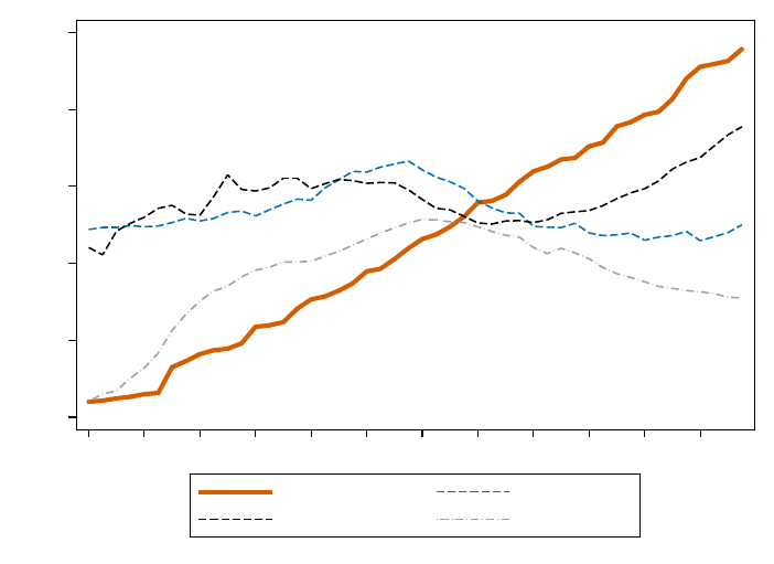
Figure 2: Non-mortgage-related Household Debt Balances This ﬁgure shows the time-series evo-

lution of non-mortgage-related debt balances. Amounts shown are in nominal terms. Source: NY

Fed CCP/Equifax.

200 400 600 800 1000 1200

Dollars, billions

2003 2004 2005 2006 2007 2008 2009 2010 2011 2012 2013 2014

Student loans Credit cards

Auto loans HELOCs

Figure 3: Aggregate Student Loan Originations This ﬁgure shows the time-series evolution of ag-

gregate student loan originations by program type. Amounts shown are in nominal terms. Source:

College Board.

0 50 100 150

Dollars, billions

2001 2002 2003 2004 2005 2006 2007 2008 2009 2010 2011 2012

Federal undergrad subsidized Federal undergrad unsubsidized

Federal undergrad PLUS Federal graduate (all)

Non-federal

Figure 4: Aggregate Pell Grant and Federal Loan Amounts This ﬁgure plots Pell Grant disburse-

ments by year as compared to total undergraduate federal student loan originations. Source: Title

IV.

0 20 40 60 80

Dollars, billions

2001 2002 2003 2004 2005 2006 2007 2008 2009 2010 2011 2012

Federal Student Loans (undergraduates only) Pell Grants

Figure 5: Per-borrower Subsidized and Unsubsidized Federal Student Loan Amounts This ﬁg-

ure shows changes in the average borrowed amounts in the subsidized and unsubsidized loan

programs. Source: IPEDS, Title IV.

3000 3500 4000 4500

Dollars

2001 2002 2003 2004 2005 2006 2007 2008 2009 2010 2011 2012

Subsidized Unsubsidized

Figure 6: Distribution of Student Loan Amounts These ﬁgures plot the distribution of student

loan amounts in the NY Fed CCP/Equifax panel in the year before (2006:Q3-2007:Q2) and after

(2007:Q3-2008:Q2) the change in the subsidized loan maximum. The maximums are marked on

the x-axis for each academic year. Source: NY Fed CCP/Equifax.

(a) Student Loan Amount in 2006-2007

5.0e+04

1.0e+05

1.5e+05

2.0e+05

Frequency

0 2625 3500 5500

(b) Student Loan Amount in 2007-2008

5.0e+04

1.0e+05

1.5e+05

Frequency

0 3500 4500 5500

Figure 7: Placebo tests This ﬁgure shows a time series (orange) of estimated ξ coeﬃcients

from equation (14) measuring the sensitivity of ∆Aid and ∆Tuition to an institution expo-

sure to each type of aid. Vertical dotted black line (year 2006) is the baseline/omitted year

in the regression. Dotted blue lines represent 95% conﬁdence intervals. For each aid type,

the gray bars show the actual mean change in program maximums, measured as the mean

of yearly cap changes times institution exposures.

(a) Subsidized loan exposure: ∆Subsidized loans

-.5

-250

250

500

Mean exposure X Δ policy cap (dollars)

2002 2004 2006 2008 2010 2012

Δ policy cap Estimated coefﬁcient ξ

(b) Subsidized loan exposure: ∆Tuition

-.5

-250

250

500

Mean exposure X Δ policy cap (dollars)

2002 2004 2006 2008 2010 2012

Δ policy cap Estimated coefﬁcient ξ

-.5

-250

250

500

Mean exposure X Δ policy cap (dollars)

2002 2004 2006 2008 2010 2012

Δ policy cap Estimated coefﬁcient ξ

(d) Unsubsidized loan exposure: ∆Tuition

-.5

-250

250

500

Mean exposure X Δ policy cap (dollars)

2002 2004 2006 2008 2010 2012

Δ policy cap Estimated coefﬁcient ξ

(e) Pell Grant exposure: ∆Pell Grants

-.5

-250

250

500

Mean exposure X Δ policy cap (dollars)

2002 2004 2006 2008 2010 2012

Δ policy cap Estimated coefﬁcient ξ

(f) Pell Grant exposure: ∆Tuition

-.5

-250

250

500

Mean exposure X Δ policy cap (dollars)

2002 2004 2006 2008 2010 2012

Δ policy cap Estimated coefﬁcient ξ

Table 1: Changes in Title IV Federal Aid Program Maximums This table shows changes to the

maximums (caps) (reported as dollar amounts) of the Federal Direct Loan and Pell Grant Program.

Y1, Y2, Y3, Y4, Grad are respectively the maximums for undergraduate freshmen, sophomores,

juniors, seniors and graduate students. (D) and (I) refers to dependent and independent students.

See Section 3 for more detail. Source: Higher Education Act, subsequent amendments and ED

appropriations.

Subsidized Loans Unsubsidized Loans Pell Grants

Year Y1 Y2 Y3/Y4 Grad Y1-Y4(D) Y1/Y2(I) Y3/Y4(I) Grad Y1-Y4

2000-01 2625 3500 5500 8500 0 4000 5000 10000 3350

2001-02 2625 3500 5500 8500 0 4000 5000 10000 3750

2002-03 2625 3500 5500 8500 0 4000 5000 10000 4000

2003-04 2625 3500 5500 8500 0 4000 5000 10000 4050

2004-05 2625 3500 5500 8500 0 4000 5000 10000 4050

2005-06 2625 3500 5500 8500 0 4000 5000 10000 4050

2006-07 2625 3500 5500 8500 0 4000 5000 10000 4050

2007-08 3500 4500 5500 8500 0 4000 5000 12000 4310

2008-09 3500 4500 5500 8500 2000 6000 7000 12000 4731

2009-10 3500 4500 5500 8500 2000 6000 7000 12000 5350

2010-11 3500 4500 5500 8500 2000 6000 7000 12000 5550

2011-12 3500 4500 5500 8500 2000 6000 7000 12000 5550

Table 2: Summary statistics This table reports summary statistics for the variables included in the

regression tables. The unit of observation is a year (t) and institution (i). The sample starts in 2002

and ends in 2012. The ∆ operator indicates annual changes (between year t and t − 1). Sample

sizes are rounded to the nearest 10 in compliance with NPSAS nondisclosure policies. Additional

detail on the variables are available in Section 4 and Appendix E.

Mean St.Dev. Min Max Count

∆StickerTuition

743.97 730.09 -2832.00 4256.00 10560

∆PellGrants

109.60 254.49 -1691.52 2144.92 10060

∆SubLoans

83.68 267.29 -1781.18 1908.91 9780

∆UnsubLoans

148.30 431.71 -3060.49 3410.32 9740

SubLoanExp

0.15 0.14 0.00 0.74 10560

UnsubLoanExp

0.27 0.21 0.00 1.00 10560

PellGrantExp

0.34 0.19 0.00 1.00 10560

SubLoanExp08

0.08 0.08 0.00 0.60 6640

UnsubLoanExp08

0.27 0.18 0.00 0.83 6640

PellGrantExp08

0.38 0.15 0.00 0.97 6640

∆InstGrant

268.56 451.99 -1672.54 2249.36 5570

∆StickerTuition

− ∆InstGrant

687.19 692.33 -3478.73 4892.03 5570

100 × ∆log(FTE

) 2.30 9.26 -47.99 53.48 9630

∆

StateFunding

11.68 1012.93 -4765.55 4795.79 9420

∆

FederalFunding

93.46 588.62 -3147.55 3346.77 9340

∆

OtherFunding

260.32 1384.37 -7436.50 8131.24 9340

∆

PrivateFunding

79.62 4348.30 -25832.35 26098.26 9340

Table 3: Baseline regression speciﬁcation The ﬁrst four columns in this table report OLS regres-

sion estimates of yearly changes in Pell Grants and subsidized/unsubsidized loan amounts per

full-time equivalent student, and sticker tuition on interactions between cross-sectional institution

exposures and yearly changes in program caps. The last column reports IV regression estimates of

the eﬀect of changes in federal loans and grants on sticker price tuition. The dependent variable

is the annual change in sticker price tuition at the institution level. Observed changes in federal

grants and loans per enrolled student are instrumented by the products of the corresponding aid

exposures and changes in program caps, as described in the text. The unit of observation is a year

(t) and institution (i). The sample starts in 2002 and ends in 2012. Sample sizes are rounded to

the nearest 10 in compliance with NPSAS nondisclosure policies. Standard errors clustered at the

institution level reported in brackets. Signiﬁcance:

∗

p < 0.1,

∗∗

p < 0.05,

∗∗∗

p < 0.01.

(1) (2) (3) (4) (5)

∆SubLoans

∆UnsubLoans

∆PellGrants

∆StickerTuition

SubLoanExp

× ∆SLCap

0.664

∗∗∗

0.146 0.056 0.587

∗∗∗

[0.12] [0.15] [0.07] [0.17]

UnsubLoanExp

× ∆USLCap

0.041

∗

0.544

∗∗∗

-0.039

∗∗∗

0.168

∗∗∗

[0.02] [0.05] [0.01] [0.04]

PellGrantExp

× ∆PGCap

-0.389

∗∗∗

-0.482

∗∗∗

1.152

∗∗∗

0.373

∗∗

[0.08] [0.12] [0.09] [0.15]

∆SubLoans

0.891

∗∗

[0.35]

∆UnsubLoans

0.243

∗∗

[0.10]

∆PellGrants

0.527

∗∗∗

[0.18]

Estimator OLS OLS OLS OLS IV

Inst&Year FE? Yes Yes Yes Yes Yes

Adj R

.07 .21 .44 .38 .

N Obs 9790 9740 10060 10570 9320

N Inst 990 990 1040 1060 970

Table 4: Regression estimates for institutional grants and enrollments This table reports OLS

regression estimates of yearly changes in institution grant expenditure per FTE, diﬀerence between

sticker price and institution grant expenditure and percentage growth rate of FTE on interactions

between cross-sectional institution exposures and yearly changes in program caps. The unit of

observation is a year (t) and institution (i). The sample starts in 2002 and ends in 2012. Sample

sizes are rounded to the nearest 10 in compliance with NPSAS nondisclosure policies. Standard

errors clustered at the institution level reported in brackets. Signiﬁcance:

∗

p < 0.1,

∗∗

p < 0.05,

∗∗∗

p < 0.01.

(1) (2) (3)

∆InstGrant

∆StickerTuition

− ∆InstGrant

100 × ∆log(FTE

)

SubLoanExp

× ∆SLCap

-0.201

∗

0.886

∗∗∗

-0.004

[0.12] [0.31] [0.00]

UnsubLoanExp

× ∆USLCap

-0.037 0.154

∗∗

-0.002

∗∗∗

[0.05] [0.07] [0.00]

PellGrantExp

× ∆PGCap

-0.330

∗∗

0.423 0.017

∗∗∗

[0.16] [0.28] [0.00]

Inst&Year FE? Yes Yes Yes

Adj R

0.31 0.17 0.08

N Obs 6290 5580 11050

N Inst 690 650 1000

Table 5: Subsamples for baseline tuition regression speciﬁcation This table reports OLS regres-

sion estimates of yearly changes in sticker tuition on interactions between cross-sectional institution

exposures and yearly changes in program caps. The unit of observation is a year (t) and institution

(i). Column 1 reproduces column 4 in Table 3 and is estimated between 2002 and 2012. The other

two columns restrict the estimation sample as noted. Sample sizes are rounded to the nearest 10 in

compliance with NPSAS nondisclosure policies. Standard errors clustered at the institution level

reported in brackets. Signiﬁcance:

∗

p < 0.1,

∗∗

p < 0.05,

∗∗∗

p < 0.01.

(1) (2) (3)

∆StickerTuition

Full sample Pre-2009 Pre-2008

SubLoanExp

× ∆SLCap

0.587

∗∗∗

0.479

∗∗∗

0.502

∗∗∗

[0.17] [0.18] [0.18]

UnsubLoanExp

× ∆USLCap

0.168

∗∗∗

0.165

∗∗∗

-0.132

[0.04] [0.05] [0.31]

PellGrantExp

× ∆PGCap

0.373

∗∗

0.396

∗

0.570

∗∗

[0.15] [0.21] [0.24]

Inst&Year FE? Yes Yes Yes

Adj R

0.38 0.40 0.38

N Obs 10570 7720 6730

N Inst 1060 1050 1050

Table 6: Regression estimates with additional controls This table reports OLS estimates of the

baseline model (Table 3) with the inclusion of additional controls. The additional cross-sectional

controls (for which coeﬃcients are not reported) are each interacted with the three changes in

program caps ∆Caps

= h∆PGCap

, ∆SLCap

, ∆USLCap

i. Changes in other sources or funding

are computed over a two year period (∆

). The unit of observation is a year (t) and institution

(i). The sample starts in 2002 and ends in 2012. Sample sizes are rounded to the nearest 10 in

compliance with NPSAS nondisclosure policies. Standard errors clustered at the institution level

reported in brackets. Signiﬁcance:

∗

p < 0.1,

∗∗

p < 0.05,

∗∗∗

p < 0.01.

(1) (2) (3)

∆StickerTuition

SubLoanExp

× ∆SLCap

0.584

∗∗

0.470

∗∗

0.452

∗∗

[0.18] [0.21] [0.20]

UnsubLoanExp

× ∆USLCap

0.165

∗∗

0.004 0.093

∗∗

[0.04] [0.06] [0.05]

PellGrantExp

× ∆PGCap

0.335

∗∗

0.176 0.119

[0.16] [0.24] [0.17]

∆

StateFunding

-0.049

∗∗

[0.01]

∆

FederalFunding

-0.005

[0.01]

∆

OtherFunding

0.001

[0.01]

∆

PrivateFunding

-0.004

∗∗

[0.00]

Inst&Year FE? Yes Yes Yes

ForProﬁt

× ∆Caps

Yes Yes Yes

Four-year

× ∆Caps

No Yes No

AdmitRate04

× ∆Caps

No Yes No

EFC04

× ∆Caps

No Yes No

Tuition04

× ∆Caps

No Yes No

Adj R

0.38 0.38 0.37

N Obs 10570 10480 8790

N Inst 1060 1040 950

Table 7: Correlation among institution characteristics This table reports a correlation matrix be-

tween institution level characteristics measured as of 2004. Standard errors clustered at the insti-

tution level reported in brackets. Signiﬁcance:

∗

p < 0.1,

∗∗

p < 0.05,

∗∗∗

p < 0.01.

SubLoanExp

UnsubLoanExp

PellGrantExp

EFC

Tuition

AdmitRate

SubLoanExp

UnsubLoanExp

0.782 1

PellGrantExp

0.197 -0.0411 1

EFC

-0.0445 0.218 -0.731 1

Tuition

0.273 0.500 -0.395 0.660 1

AdmitRate

-0.145 -0.322 0.255 -0.424 -0.591 1

Table 8: Sensitivity of aid exposures to institution attributes This table expands on the base-

line results of Table 3 by allowing the coeﬃcients to vary across these institution characteristics: a

dummy for private institutions, a dummy for 4-year programs, the 2004 levels of tuition and aver-

age EFC (both in thousands). See notes to Table 3 for more details. Sample sizes are rounded to

the nearest 10 in compliance with NPSAS nondisclosure policies. Standard errors clustered at the

institution level reported in brackets. Signiﬁcance:

∗

p < 0.1,

∗∗

p < 0.05,

∗∗∗

p < 0.01.

(1) (2) (3)

∆StickerTuition

SubLoanExp

× ∆SLCap

0.264 0.546

∗∗

0.603

∗∗

[0.28] [0.17] [0.17]

UnsubLoanExp

× ∆USLCap

0.170

∗∗

-0.173 0.185

∗∗

[0.04] [0.11] [0.04]

PellGrantExp

× ∆PGCap

0.384

∗∗

0.506

∗∗

0.541

∗

[0.15] [0.16] [0.32]

SubLoanExp

× ∆SLCap

×Private

0.304

∗∗

[0.11]

SubLoanExp

× ∆SLCap

×FourYear

-0.321

∗∗

[0.11]

SubLoanExp

× ∆SLCap

×Tuition04

0.022

∗∗

[0.01]

SubLoanExp

× ∆SLCap

×EFC04

-0.015

[0.01]

UnsubLoanExp

× ∆USLCap

×Private

0.061

[0.04]

UnsubLoanExp

× ∆USLCap

×FourYear

-0.047

[0.04]

UnsubLoanExp

× ∆USLCap

×Tuition04

0.009

∗∗

[0.00]

UnsubLoanExp

× ∆USLCap

×EFC04

0.000

[0.00]

PellGrantExp

× ∆PGCap

×Private

-0.040

[0.13]

PellGrantExp

× ∆PGCap

×FourYear

0.041

[0.14]

PellGrantExp

× ∆PGCap

×Tuition04

-0.010

[0.01]

PellGrantExp

× ∆PGCap

×EFC04

-0.007

[0.02]

Inst&Year FE? Yes Yes Yes

Adj R

0.38 0.38 0.38

N Obs 10570 10570 10570

N Inst 1060 1060 1060

Table 9: Years of Federal Loan, Pell Grant, and Tuition increases for For-Proﬁt and Not-for-Proﬁt

institutions These tables regress annual changes in federal subsidized and unsubsidized loans, Pell

Grants, and sticker price tuition against year dummies. The omitted dummy is for the year 2006.

The Year = 2008,09,10 is a dummy varaible corresponding to those years, which is when the federal

aid cap changes take eﬀect. Standard errors clustered at the institution level reported in brackets.

Signiﬁcance:

∗

p < 0.1,

∗∗

p < 0.05,

∗∗∗

p < 0.01.

For-Proﬁts

∆PellGrants

∆SubLoans

∆UnsubLoans

∆StickerTuition

Year = 2002 178

∗∗

[14] -74

∗∗

[19] -246

∗∗

[29] 25 [49]

Year = 2003 110

∗∗

[13] -64

∗∗

[17] -194

∗∗

[27] 226

∗∗

[46]

Year = 2004 -28

∗∗

[12] -84

∗∗

[17] -210

∗∗

[26] 36 [25]

Year = 2005 -112

∗∗

[14] -115

∗∗

[18] -252

∗∗

[27] 86

∗∗

[25]

Year = 2007 -35

∗∗

[14] -50

∗∗

[18] -317

∗∗

[27] 83

∗∗

[25]

Year = 2008 89

∗∗

[14] 460

∗∗

[20] -117

∗∗

[27] 205

∗∗

[27]

Year = 2009 252

∗∗

[14] -53

∗∗

[18] 670

∗∗

[29] 269

∗∗

[29]

Year = 2010 728

∗∗

[17] -264

∗∗

[18] -485

∗∗

[27] 269

∗∗

[29]

Year = 2011 106

∗∗

[16] -215

∗∗

[18] -576

∗∗

[28] 88

∗∗

[28]

Year = 2012 -485

∗∗

[18] -249

∗∗

[19] -374

∗∗

[30] -102

∗∗

[30]

Constant 85

∗∗

[8] 164

∗∗

[10] 371

∗∗

[15] 487

∗∗

[15]

∆PellGrants

∆SubLoans

∆UnsubLoans

∆StickerTuition

Year = 2008,09,10 386

∗∗

[8] 148

∗∗

[9] 272

∗∗

[13] 212

∗∗

[16]

Constant 50

∗∗

[2] 67

∗∗

[2] 126

∗∗

[4] 523

∗∗

[5]

Inst FE? Yes Yes Yes Yes

N Obs 18750 16980 16760 16880

N Inst 2050 1910 1900 2090

Not-for-Proﬁts

∆PellGrants

∆SubLoans

∆UnsubLoans

∆StickerTuition

Year = 2002 -106

∗∗

[7] -260

∗∗

[9] -513

∗∗

[12] -164

∗∗

[12]

Year = 2003 -157

∗∗

[7] -165

∗∗

[9] -456

∗∗

[12] -38

∗∗

[13]

Year = 2004 -229

∗∗

[7] -174

∗∗

[9] -477

∗∗

[12] 60

∗∗

[14]

Year = 2005 -252

∗∗

[7] -201

∗∗

[9] -483

∗∗

[12] 33

∗∗

[13]

Year = 2007 -262

∗∗

[7] -257

∗∗

[9] -588

∗∗

[12] 6 [12]

Year = 2008 -161

∗∗

[7] -22

∗∗

[10] -445

∗∗

[13] 46

∗∗

[12]

Year = 2009 -76

∗∗

[7] -223

∗∗

[9] 10 [16] 79

∗∗

[12]

Year = 2010 294

∗∗

[9] -186

∗∗

[9] -452

∗∗

[14] 54

∗∗

[13]

Year = 2011 -32

∗∗

[8] -237

∗∗

[10] -688

∗∗

[14] 36

∗∗

[13]

Year = 2012 -315

∗∗

[8] -241

∗∗

[9] -560

∗∗

[13] 90

∗∗

[12]

Constant 260

∗∗

[5] 292

∗∗

[5] 630

∗∗

[7] 618

∗∗

[7]

∆PellGrants

∆SubLoans

∆UnsubLoans

∆StickerTuition

Year = 2008,09,10 159

∗∗

[4] 16

∗∗

[4] 94

∗∗

[7] 54

∗∗

[7]

Constant 118

∗∗

[1] 134

∗∗

[1] 241

∗∗

[2] 623

∗∗

[2]

Inst FE? Yes Yes Yes Yes

N Obs 39420 38390 37830 37850

N Inst 3550 3440 3420 3630

Appendix

A Proof of model propositions

Proof of Proposition 1 Letting λ be the Lagrange multiplier on the capacity constraint, the ﬁrst order conditions are:

−γN

−1

qδD

q,U

+ (1 − γ)N

−1

q,U

− (1 − γ)(t

q,U

− c)δD

q,U

− λδD

q,U

= 0 (15)

−γN

−1

q(δ + ω)D

q,C

+ (1 − γ)N

−1

q,C

− (1 − γ)(t

q,C

− c)(δ + ω)D

q,C

− λ(δ + ω)D

q,C

= 0 (16)

for q = q

, q

, where we have used the observation that

∂D

q,U

∂t

q,U

= δD

q,U

and

∂D

q,C

∂t

q,C

= (δ + ω)D

q,C

. When λ > 0 (i.e. the

constraint binds) this gives us the solutions above.

Proof of Proposition 2 We ﬁrst note that:

∂t(q, n)

∂B

1 − γ

(17)

for q = q

, q

and n = n

, n

. We can solve implicitly for λ

by taking the derivative of the constraint D

+ D

= N

with respect to B.

∂D

∂B

∂D

∂B

= 0. (18)

Notice that:

∂D

∂B

= −

δD

1 − γ

∂λ

∂B

(19)

∂D

∂B

= −

(δ + ω)D

1 − γ

∂λ

∂B

+ ωD

(20)

This gives us:

δD

+ (δ + ω)D

1 − γ

∂λ

∂G

= ωD

(21)

(1 − γ)D

δD

+ (δ + ω)D

(22)

(1 − γ)D

δN + D

(23)

Thus we have that:

∂t(q, n)

∂B

δN + D

> 0 (24)

Proof of Proposition 3 We use the expression for

∂t(q,n)

∂B

from above to write that:

∂

∂s

∂t

∂B

(δN + D

ω)ω

∂D

∂s

− D

ωω

∂D

∂s

(δN + D

ω)

(25)

δNω

(δN + D

ω)

∂D

∂s

(26)

Thus, showing the ﬁrst comparative static is equivalent to showing that

∂D

∂s

> 0. We compute:

∂D

∂s

= q

∂D

L,U

∂s

+ (1 − q)

∂D

H,U

∂s

(27)

= −q

L,U

1 − s

− qδD

L,U

∂t

L,U

∂s

− (1 − q)

H,U

1 − s

− (1 − q)δD

H,U

∂t

H,U

∂s

(28)

= −

1 − s

−

δD

1 − γ

∂λ

∂s

(29)

and likewise:

∂D

∂s

−

(δ + ω)D

1 − γ

∂λ

∂s

(30)

Then we solve for λ

by again taking derivatives of the constraint:

∂D

∂s

∂D

∂s

= 0 (31)

⇒ −

1 − s

1 − γ

∂λ

∂s

δD

+ (δ + ω)D

(32)

⇒ λ

(1 − γ)(D

/s − D

/(1 − s))

δD

+ (δ + ω)D

(33)

⇒ λ

(1 − γ)(D

− N)

s(1 − s)



δN + ωD



(34)

Thus:

∂D

∂s

> 0 ⇔

(δ + ω)

1 − γ

(1 − γ)(D

− N)

s(1 − s)(δN + ωD

)

(35)

⇔ 1 − s >

(δ + ω)(D

− N)

δN + ωD

(36)

Since the RHS is negative, this inequality is always true.

Sensitivity of tuition response to for-proﬁt motive Here we show that

∂

∂γ

∂t

∂B

< 0 ⇔

H,C

δD

H,U

+ (δ + ω)D

H,C

δD

+ (δ + ω)D

(37)

We use the expression for

∂t(q,n)

∂B

from above to write that:

∂

∂γ

∂t

∂B

δNω

(δN + D

ω)

∂D

∂γ

(38)

and thus that we want to show that:

∂D

∂γ

< 0. We compute the derivatives of the demand function with respect to

γ as follows:

∂D

q,U

∂γ

= −δD

q,U



−

q + λ

(1 − γ)

1 − γ

∂λ

∂γ



(39)

∂D

q,C

∂γ

= −(δ + ω)D

q,C



−

q + λ

(1 − γ)

1 − γ

∂λ

∂γ



(40)

We use these to solve for λ

∂D

H,U

∂γ

∂D

L,U

∂γ

∂D

H,C

∂γ

∂D

H,C

∂γ

= 0

⇒

δ(D

H,U

+ λ) + D

L,U

+ λ)) + (δ + ω)(D

H,C

+ λ) + D

L,C

+ λ))

(1 − γ)

∂λ

∂γ

1 − γ

δD

+ (δ + ω)D

⇒ λ

δ(D

H,U

+ λ) + D

L,U

+ λ)) + (δ + ω)(D

H,C

+ λ) + D

L,C

+ λ))

(1 − γ)



δD

+ (δ + ω)D



⇒ λ

δD

H,U

+ (δ + ω)D

H,C

δD

+ (δ + ω)D

+ λ

1 − λ

δD

L,U

+ (δ + ω)D

L,C

δD

+ (δ + ω)D

+ λ

1 − λ

(41)

Thus:

∂D

∂γ

= −(δ + ω)



1 − γ

∂λ

∂γ

− D

H,C

+ λ

(1 − γ)

− D

L,C

+ λ

(1 − γ)



(42)

∂D

∂γ

< 0 ⇔ λ

H,C

+ λ

1 − γ

L,C

+ λ

1 − γ

(43)

⇔

δD

H,U

+ (δ + ω)D

H,C

δD

+ (δ + ω)D

H,C

(44)

where the ﬁnal implication follows from the fact that the left and right sides are both weighted sums of

+λ

1−γ

and

+λ

1−γ

where the weights sum to 1, and q

> q

B Overview of the postsecondary education industry

This Appendix provides basic facts about the postsecondary education industry. As discussed above, average un-

dergraduate per student tuition nearly doubled between 2001 and 2012, from about $6,950 to more than $10,000 in 2012

dollars (Figure 1), corresponding to an average real rate increase of 3.5% per year.

These overall trends in college tuition mask signiﬁcant variation within the postsecondary education sector. Tuition

at postsecondary educational institutions varies widely depending on the type of degree the institution oﬀers (four-year

bachelor’s degrees, two-year associate’s degrees, or certiﬁcates generally requiring less than two years of full time study)

and by the type of governance it operates under (for example, non-proﬁt or for-proﬁt).

In the 2011-2012 school year, there were 10.7 million undergraduate students enrolled at four-year institutions, and

7.5 million students enrolled at two-year institutions (see Figure 8). Four-year institutions also enrolled an additional 2.8

million graduate students, though we focus mainly on undergraduate loan amounts and tuition in this paper. Four-year

institutions, which include public state universities (60% of enrollment in 2012), private non-proﬁt research universities

and liberal arts colleges (29%), and private for-proﬁt institutions (11%), rely on a combination of revenue sources, from

government appropriations to tuition revenue to other revenue (mostly private endowments and gifts). The two-year

sector is almost entirely dominated by public two-year colleges, also known as community colleges, which enroll about

95% of all two-year students. Tuition at these colleges is low, averaging just $2,600 in 2012. Most of the revenue (70%) of

these colleges instead comes from government sources.

Finally, in addition to the 20.4 million students enrolled at degree-granting institutions (two-year and four-year

institutions) in 2012, another 572,000 were enrolled at Title IV “less-than-two-year” institutions. These institutions are

mostly vocational schools in ﬁelds such as technology, business, cosmetology, hair styling, photography, and fashion.

In contrast to the degree-granting institutions, the majority of these institutions are private for-proﬁt institutions and

tuition revenue makes up the majority of their funding.

The above numbers only cover Title IV institutions, but many for-proﬁt institutions exist that are not Title IV-

eligible.

Data on these institutions is hard to ﬁnd since they are not tracked by the US Department of Education, but

All public institutions are eligible for Title IV. Other institutions must meet certain qualiﬁcations such as being li-

censed, accredited from a Nationally Recognized Accrediting Agency (NRAA), and meeting standards of administrative

Cellini and Goldin (2014) construct a dataset using administrative data from ﬁve states, and show that, after controlling

for observables, tuition at Title-IV-eligible for-proﬁt institutions are 75% higher than comparable non-Title-IV-eligible

for-proﬁt institutions.

C Additional earnings calls transcripts

In this Section we provide additional passages taken from earnings calls of the Apollo Group discussing the changes

in federal student aid maximums.

<Q - Mark Marostica>: My question ﬁrst relates to Brian’s comment on the national pricing strategy, and

I was wondering if you can give us some more speciﬁcs around that and whether or not you are actually

planning to lower prices as part of that.

<A - Brian Mueller>: It is something that we are considering. I have talked about it the last couple

of conferences we’ve attended. We have a very unique opportunity in July. Loan limits go up for ﬁrst

and second level students, which is fairly long overdue. By the time we get to July I am estimating that

upwards of 70% of all students who are studying at the University of Phoenix at the level one and level

two at those levels will be at Axia College at Axia College tuition rates. So there will be some room for

us to raise tuition there from maybe 265 to 295 and from 285 to maybe 310, without putting a burden on

students from a standpoint of out-of-pocket expense. At the graduate level there is a lot of room. We are

actually quite a bit under the competition in our graduate programs, and there is a lot of room from a Title

IV standpoint so that, again, we wouldn’t put a burden on students from an out-of-pocket expense.

Source: Apollo Education Group, 2006:Q4 Earnings Call, accessed from Bloomberg LP Transcripts.

<Q - Mark Hughes>: And then any early view on whether Axia, with the price increase there aﬀecting

start levels in May?

<A - Brian Mueller> Whether it’s aﬀecting start levels in May?

<Q - Mark Hughes>: Right. 10% increase in tuition. Is anybody balking at that, or trends steady?

<A - Brian Mueller>: No, thank you for asking that. No, because loan limits are raised on July 1, for level

1 and 2 students. And so students know as they go in if they’re going to have enough title IV dollars to

cover the cost of their tuition, so, no, it’s not impacting new student starts.

Source: Apollo Education Group, 2007:Q2 Earnings Call, accessed from Bloomberg LP Transcripts.

<Q - Brandon Dobell>: One ﬁnal one. Maybe as you think about discounting, at least the philosophy

around aﬀordability, pricing, discounting across the diﬀerent brands or diﬀerent programs, maybe, Brian,

if you could speak to, has there been any change in terms of how you guys think about that? Do you think

that discounting generates the wrong type of student or the right type of student, or how ﬂexible do you

think it will be going forward in terms of how you think about aﬀordability issues?

<A - Brian Mueller>: We’re not changing our thinking about that. It’s really clear what’s going on in

the country economically, with the middle class getting squeezed. People don’t have disposable income

to spend for private school education but they understand its impact on their long-term career so they’re

willing to borrow the money at really good rates from a Title IV standpoint. And so if you can build your

operations to the point that you can be proﬁtable and keep those tuition rates inside Title IV loan limits

you’re going to do positive things with regards to retention, which will oﬀset maybe the 4 to 6% increases

that we would have gotten in the past.

Source: Apollo Education Group, 2007:Q2 Earnings Call, accessed from Bloomberg LP Transcripts.

D Stock market event study analysis

Here we discuss stock market responses of publicly traded for-proﬁt institutions to the three legislative changes

discussed in Section 3. Table A1 reports event studies for abnormal returns over 3-day windows surrounding the passage

of the three legislative changes to the HEA. Fourteen for-proﬁt education companies were publicly traded around at least

one of these legislative changes (and eight across all changes), including the Apollo Education Group among others. The

capacity and ﬁnancial responsibility (e.g., default rates of graduates in excess of 25% for three consecutive years, or a

one-year default rate in excess of 40%, are grounds for losing Title IV status).

cumulative abnormal returns are computed as each stock’s excess return to the CRSP index returns, summed over the

3-day event window. We then calculate the (market cap) weighted and unweighted average of the cumulative abnormal

returns of the eight publicly traded for-proﬁt institutions to the index.

In the top panel of Table A1, we see that average 3-day cumulative abnormal returns around the 2006 re-authorization

of HEA, which increased the subsidized loan limits for freshman and sophomores, were 3.64% and 2.9% under the value-

and equally-weighted market benchmarks, respectively. The abnormal returns are statistically signiﬁcant and econom-

ically large. As shown in the middle panel, three-day cumulative abnormal returns surrounding the 2007 legislative

passage that increased Pell Grant amounts were 2.17% and 2.22%, respectively. Finally, we consider two separate event

windows for the passing of the Ensuring Equal Access to Student Loans Act of 2008 which increased unsubsidized

borrowing amounts.

Depending on the exact window used, abnormal returns on the for-proﬁt institution portfolio

ranged between 4.8% and 3.3%.

In sum, we ﬁnd evidence that the passage of three pieces of legislation were associated with sizable abnormal stock

market responses for the portfolio of publicly traded for-proﬁt institutions. The nearly 10% abnormal return is consistent

with the fact that students at for-proﬁt institutions rely heavily on federal student aid to fund their education. In addition,

anecdotal evidence also supports the view that changes in Title-IV programs boosted tuition at these institutions.

Table A1: Stock Market Reactions to Changes in Federal Aid Policy This table reports 3-day cu-

mulative abnormal returns for a portfolio of 14 publicly traded for-proﬁt universities surrounding

dates of legislative passage to changes in Federal Aid Policy. Returns are computed in excess of the

CRSP index on a value-weighted and equal-weighted basis.

Event Date Mkt Weights Policy Event Window Mean Cum.

Abnormal

Ret.

Z score

Congress reauthorized the

Higher Education Act

2/1/2006 v Sub./Unsub. Loans (-1,+1) 3.64% (3.216)

e Sub./Unsub. Loans (-1,+1) 2.90% (2.545)

College Cost Reduction

and Access Act Passes

Congress

9/7/2007 v Pell Grants (-1,+1) 2.17% (2.204)

e Pell Grants (-1,+1) 2.22% (2.242)

Ensuring Equal Access to

Student Loans Act of 2008

is passed by the Senate

4/30/2008 v Unsub. Loans (-1,+1) 4.86% (2.570)

e Unsub. Loans (-1,+1) 4.80% (2.480)

Ensuring Equal Access to

Student Loans Act of 2008

is passed by Congress

5/1/2008 v Unsub. Loans (-1,+1) 3.30% (1.752)

e Unsub. Loans (-1,+1) 3.62% (1.933)

E Data detail

This Appendix complements Section 4 in providing a more detailed data description. The data used in the empirical

analysis throughout this paper comes from three sources: IPEDS, Title IV, and NPSAS. We provide institutional details

on each. We then describe in detail the variables we constructed using the data from each of these sources.

Survey Data: The IPEDS survey covers seven areas: institutional characteristics, institutional prices, enrollment,

student ﬁnancial aid, degrees and certiﬁcates conferred, student retention and graduation rates, and institutional hu-

On April 30, 2008 the Senate passed the Act, after already having received approval by the House. However, the

Senate’s approving vote included some changes that had to be subsequently ratiﬁed by the House. Thus, the bill essen-

tially passed on April 30, 2008, but the changes made by the Senate were not voted on, and subsequently passed by the

House, until May 1, 2008. For completeness, we estimate three-day abnormal returns around both event dates, though

the two event window obviously overlap on one day.

man resources and ﬁnances. While IPEDS is the most comprehensive dataset on postsecondary education available,

because it is based on surveys of administrators, it is not always suﬃciently detailed or reliable for our purposes. For

measures of federal aid at the institutional level, we found that the ﬁgures contained in the IPEDS ”Student Financial

Aid” survey did not meet our needs for a couple reasons. First, the survey restricts the universe to aid amounts for

”full-time ﬁrst-time degree-seeking undergraduates,” which is not our student population of interest; second, in part

because of this restriction, the survey has been labeled as the most burdensome of surveys (Government Accountability

Oﬃce (2010)); and third, until recently, the survey did not distinguish between federal loans and other loans, and still

does not distinguish between subsidized and unsubsidized loans, which makes our identiﬁcation more diﬃcult.

Title IV data serve as our primary data source for measuring federal loans and pell grants at the institution level.

While we considered also using IPEDS to obtain these measures, we ultimately found a number of reasons to look to the

Title IV data. One of the reasons is that the IPEDS measures of ﬁnancial aid are contained in the “Student Financial Aid”

survey, which is considered by most educational administrators to be the most burdensome of the IPEDS surveys (Gov-

ernment Accountability Oﬃce (2010)). This is likely because it requires administrators to estimate the total amount of

aid and number of recipients within a speciﬁc IPEDS-deﬁned universe of students, ‘’full-time ﬁrst-time degree-seeking

undergraduates.” Restricting to this universe may be diﬃcult for some institutions depending on what data sources

they pull from to complete the IPEDS surveys. Thus, these data are less reliable than those obtained from the less-

burdensome collection of published tuition levels and enrollment numbers. Second, this universe is not necessarily

representative of the entire undergraduate body. Third, until recently, IPEDS did not distinguish between federal loans

and other loans, and still does not distinguish between subsidized and unsubsidized loans, which makes our identiﬁca-

tion more diﬃcult. We describe the beneﬁts of the Title IV data relative to the IPEDS data in Section 4 in the main body

of the text.

Sample: Our sample begins in the 2000-2001 school year, the ﬁrst year that the tuition sticker price survey from

IPEDS more or less takes the current form. We end our sample in 2011-2012, since in 2012-2013, changes to graduate

ﬁnancial aid occur that may interfere with our identiﬁcation. IPEDS and NPSAS data are reported at institution level

(UNITID), while Title IV is reported at the OPEID level. This is because there may be multiple UNITIDs associated to

one OPEID, as branches (UNITID) of the same institution are sometimes surveyed separately. Our regressions are done

at the OPEID level, where when we are using averages of variables in IPEDS, we take enrollment-weighted averages of

the UNITIDs.

Sticker-Price Tuition: Our main dependent variable is yearly changes in the sticker-price tuition at the institutional

level. This data comes from the IPEDS Student Charges survey. For full academic-year programs, we use the sum of the

out-of-state average tuition for full-time undergraduates and the out-of-state required fees for full-time undergraduates.

For other programs, we use the published tuition and fees for the entire program. For public universitites we use out-

of-state tuition rather than average tuition to abstract from variation driven by changing fractions of in-state versus

out-of-state students. We generally ﬁnd that the in-state and out-of-state diﬀerences are highly correlated.

Enrollment: Enrollment can be measured both as headcount and full-time equivalent students. In general, we use

an IPEDS formula to calculate a full-time-equivalent (FTE) enrollment measure. In certain cases though, we use total

headcounts from the IPEDS enrollment survey, which are available by student level and attendance status.

Federal Loan and Grant Usage: For federal loan and grant totals, we rely on Title IV administrative data rather than

the student ﬁnancial aid survey from IPEDS, which appears to be somewhat unreliable as it is survey based. Title IV data

contains the number of recipients, and total dollar amount of loans originated or grants disbursed for each institution

and each of subsidized loans, unsubsidized loans, and Pell Grants. We only consider undergraduate policy changes and

tuition in this paper, so we would want these amounts to be for undergraduates only. However, Title IV data does not

break out undergraduate and graduate loans separately until 2011. Pell Grants are only available to undergraduates,

so are not aﬀected. Since imputation of an undergraduate measure requires making several assumptions, our preferred

measure of loan and grant usage at an institution is just the total dollar amount scaled by the FTE count of the university.

We also report results for robustness when we scale the total dollar amount by the total enrollment count. Finally, also

for robustness, we make an attempt to impute an undergraduate measure as follows: Since the maximum subsidized

loan amount changes only for undergraduates in our sample, we assume a constant average graduate loan amount

over time,

conditional on borrowing. In addition, we assume that the fraction of all subsidized loan borrowers at an

institution who are graduate students also does not change, γ

. To calculate

and γ

, we take the averages of the 2011

and 2012 values.

For prior years, given the total subsidized loan amount S

, we calculate the undergraduate dollar

amount borrowed as: S

− γ

. We then scale this measure by total undergraduate enrollment.

Exposures: We calculate exposures using conﬁdential NPSAS data as described in Section 4.3.

Net Tuition and Institutional Grants: Our institutional grant data comes from the IPEDS Finance Survey, which

records as an expenditure item total grant dollars spent on scholarships and fellowships. We scale this measure by the

FTE enrollment. We compute net tuition by subtracting institutional grants per FTE from sticker price.

Financing Controls: We follow the Delta Cost Project data in separating revenue data into a few main parts. The

ﬁrst is net tuition revenue, as described above. The next is federal funding, excluding Pell Grants. The third is state (and

local) funding through appropriations and contracts. The fourth is private funding (from donations, or endowment

investment income), and the ﬁfth is revenue from auxiliary operations (e.g. hospitals, dormitories). We use changes in

these amounts, scaled by FTE enrollment, as controls in our regressions.

Other Controls: Average EFC comes from NPSAS data, and the admission rate comes from IPEDS.

F Additional robustness tests

Using 2008 NPSAS exposures: In the baseline speciﬁcation we measure institution exposures using the 2004

NPSAS wave, the closest available wave that still predates the changes in loan (and most of the grant) maximums.

Despite the results in Table 3, one may worry about the time gap between when the exposures are computed and when

the policy changes take place. In Table A2 we re-estimate the baseline speciﬁcation using exposures computed from

2008 NPSAS for robustness. Aid sensitivities to changes in the institution-speciﬁc program aid maximums as of 2008

maximums (columns 1-3) are very similar to the 2004 ones, with the exception of the subsidized loan sensitivity response

to the subsidized loan maximums, which increases to 1.25 from .7 in Table 3. Subsidized loan maximums are increased in

2008, so that the 2008 subsidized loan exposure is measured at the post-policy maximum amounts. To the extent that not

all students fully expanded their borrowing (as suggested by comparing the 2004-08 subsidized exposures in Table 2 and

the loading in Table 3), the sensitivity of 2008 to 2004 subsidized exposures drops, resulting in a higher point estimate

in column 3. Sticker tuition displays a very similar sensitivity to the institution-level change in program maximums

(compare columns 4 in Tables 3 and A2), although the point estimate on Pell Grants is less precisely estimated (t-stat =

1.66). In Table A3, we repeat the IV estimates of Table ?? using exposures computed as of 2008 NPSAS and obtain very

similar results, except for a lower sensitivity of sticker tuition to subsidized loans owing to the overstated pre-policy

exposure discussed above.

Dependent variables in logarithms: Because changes in federal aid policies aﬀected dollar levels, rather than

percentage changes, of the program maximums, the dependent variables in our baseline speciﬁcation are expressed

in dollar changes. In Table A4 we re-estimate the speciﬁcation with the dependent variable expressed in logarithmic

changes. While this speciﬁcation does not directly match the policy change, it can be informative about the magnitude

of percentage eﬀects of the changes in program caps. Starting with the percentage change response of aid levels, Pell

amounts (column 1) now load with an incorrect (negative) sign on changes in Pell caps.

Subsidized and unsubsidized

loans (columns 2 and 3) load positively on changes in their respective caps and negatively on the Pell Grant caps suggest-

ing substitution from loans to grants, as in the baseline speciﬁcation in dollar changes. Finally, in terms of percentage

changes in tuition, a $100 increase in the program caps resulted in .4%, .2% and .1% (statistically signiﬁcant) increases,

respectively, for Pell Grants, subsidized, and unsubsidized loans.

We drop institutions from our sample where the 2011 and 2012 values diﬀer signiﬁcantly.

This may owe to the percentage-change speciﬁcation along with the fact that, because of the program design, Pell

Grant exposures include all recipients receiving a positive, rather than only those at the program maximums as it is the

case for subsidized and unsubsidized loans.

Table A2: Baseline regression speciﬁcation using 2008 NPSAS exposures This table replicates

Table 3 using NPSAS aid exposures as of 2008 as opposed to 2004 ones. See notes to Table 3 for

more details. Sample sizes are rounded to the nearest 10 in compliance with NPSAS nondisclosure

policies. Standard errors clustered at the institution level reported in brackets. Signiﬁcance:

∗

p <

0.1,

∗∗

p < 0.05,

∗∗∗

p < 0.01.

(1) (2) (3) (4) (5)

∆SubLoans

∆UnsubLoans

∆PellGrants

∆StickerTuition

SubLoanExp08

× ∆SLCap

1.223

∗∗∗

0.106 0.108 0.609

∗∗∗

[0.11] [0.16] [0.08] [0.23]

UnsubLoanExp08

× ∆USLCap

0.030 0.650

∗∗∗

-0.057

∗∗∗

0.233

∗∗∗

[0.02] [0.04] [0.01] [0.04]

PellGrantExp08

× ∆PGCap

-0.346

∗∗∗

-0.466

∗∗∗

0.997

∗∗∗

0.283

[0.08] [0.15] [0.09] [0.17]

∆SubLoans

0.891

∗∗

[0.35]

∆UnsubLoans

0.243

∗∗

[0.10]

∆PellGrants

0.527

∗∗∗

[0.18]

Inst&Year FE? Yes Yes Yes Yes Yes

Adj R

0.08 0.23 0.48 0.39 -0.45

N Obs 13610 13540 14000 14500 9320

N Inst 1340 1350 1410 1420 970

Table A3: IV regression speciﬁcation using 2008 NPSAS exposures This table replicates Table ??

using NPSAS aid exposures as of 2008 as opposed to 2004 ones. See notes to Table ?? for more

details. Sample sizes are rounded to the nearest 10 in compliance with NPSAS nondisclosure poli-

cies. Standard errors clustered at the institution level reported in brackets. Signiﬁcance:

∗

p < 0.1,

∗∗

p < 0.05,

∗∗∗

p < 0.01.

(1) (2)

∆StickerTuition

∆PellGrants

0.270

∗

0.559

∗∗

[0.16] [0.18]

∆SubLoans

0.502

∗∗

[0.22]

∆UnsubLoans

0.352

∗∗

[0.07]

Inst&Year FE? Yes Yes

N Obs 13110 13110

N Inst 1340 1340

Figure 8: Enrollments, Sticker Tuition and Revenue by Program Type These ﬁgures plot total

enrollment, average sticker price, and average revenues per student for institutions, depending on

the type of program oﬀered in the 2011-2012 school year. Source: IPEDS.

(a) Total undergraduate enrollment by institution pro-

gram type (millions)

0 2 4 6 8 10

Millions

4-Year 2-Year Less-than-2-Year

(b) Average sticker price by institution program type

0 5,000 10,000 15,000

Dollars

4-Year 2-Year Less-than-2-Year

type

0 10,000 20,000 30,000

Dollars

4-Year 2-Year Less-than-2-Year

Net Tuition Gov. Appropriations and Contracts

Other

Table A4: Baseline regression speciﬁcation with dependent variables in logarithmic changes

This table replicates Table 3, but uses percentage changes in the dependent variables rather than

changes in absolute terms. See notes to Table 3 for more details. Sample sizes are rounded to the

nearest 10 in compliance with NPSAS nondisclosure policies. Standard errors clustered at the

institution level reported in brackets. Signiﬁcance:

∗

p < 0.1,

∗∗

p < 0.05,

∗∗∗

p < 0.01.

(1) (2) (3) (4)

∆ logPellGrants

∆ logSubLoans

∆ logUnsubLoans

∆ logStickerTuition

SubLoanExp

× ∆SLCap

0.009

∗

0.009

∗

0.000 0.002

∗

[0.00] [0.01] [0.01] [0.00]

UnsubLoanExp

× ∆USLCap

-0.003

∗∗∗

0.001 0.014

∗∗∗

0.001

∗∗∗

[0.00] [0.00] [0.00] [0.00]

PellGrantExp

× ∆PGCap

-0.016

∗∗∗

-0.017

∗∗∗

-0.026

∗∗∗

0.004

∗∗

[0.00] [0.00] [0.01] [0.00]

Inst&Year FE? Yes Yes Yes Yes

Adj R

0.49 0.13 0.19 0.04

N Obs 10040 9740 9730 10480

N Inst 1040 990 990 1060