Opportun Kristen NBER WORKING PAPER SERIES HOW DID

The Opportun

Wahlers, Kristen

NBER WORKING PAPER SERIES

HOW DID COVID-19 AND STABILIZATION POLICIES

AFFECT SPENDING AND EMPLOYMENT?

A NEW REAL-TIME ECONOMIC TRACKER BASED ON PRIVATE SECTOR DATA

Raj Chetty

John N. Friedman

Nathaniel Hendren

Michael Stepner

The Opportunity Insights Team

Working Paper 27431

http://www.nber.org/papers/w27431

NATIONAL BUREAU OF ECONOMIC RESEARCH

1050 Massachusetts Avenue

Cambridge, MA 02138

June 2020

A preliminary draft of this paper was previously circulated as “Real-Time Economics: A New

Platform to Track the Impacts of COVID-19 on People, Businesses, and Communities Using

Private Sector Data.” We thank Gabriel Chodorow-Reich, Jason Furman, Xavier Jaravel,

Lawrence Katz, Emmanuel Saez, Ludwig Straub, and Danny Yagan for helpful comments. We

also thank the corporate partners who provided the underlying data used in the Economic

Tracker, who as of this version include: Affinity Solutions (especially Atul Chadha and Arun

Rajagopal), Burning Glass (especially Anton Libsch and Bledi Taska), Earnin (especially Arun

Natesan and Ram Palaniappan), Homebase (especially Ray Sandza and Andrew Vogeley), Intuit

(especially Christina Foo and Krithika Swaminathan), Womply (especially Toby Scammell and

Ryan Thorpe), and Zearn (especially Billy McRae and Shalinee Sharma). We are very grateful to

Ryan Rippel of the Gates Foundation for his support in launching this project and to Gregory

Bruich for early conversations that helped spark this work. The work was funded by the Chan-

Zuckerberg Initiative, Bill & Melinda Gates Foundation, Overdeck Family Foundation, and

Andrew and Melora Balson. The project was approved under Harvard University IRB 20-0586.

†The Opportunity Insights Economic Tracker Team consists of Matthew Bell, Gregory Bruich,

Tina Chelidze, Lucas Chu, Westley Cineus, Sebi Devlin-Foltz, Michael Droste, Shannon Felton

Spence, Dhruv Gaur, Federico Gonzalez, Rayshauna Gray, Abby Hiller, Matthew Jacob, Tyler

Jacobson, Margaret Kallus, Laura Kincaide, Cailtin Kupsc, Sarah LaBauve, Maddie Marino, Kai

Matheson, Kate Musen, Danny Onorato, Sarah Oppenheimer, Trina Ott, Lynn Overmann, Max

Pienkny, Jeremiah Prince, Daniel Reuter, Peter Ruhm, Emanuel Schertz, Kamelia Stavreva,

James Stratton, Elizabeth Thach, Nicolaj Thor, Amanda Wahlers, Kristen Watkins, Alanna

Williams, David Williams, Chase Williamson, Shady Yassin, and Ruby Zhang.

NBER working papers are circulated for discussion and comment purposes. They have not been

peer-reviewed or been subject to the review by the NBER Board of Directors that accompanies

official NBER publications.

paragraphs, may be quoted without explicit permission provided that full credit, including ©

notice, is given to the source.

How Did COVID-19 and Stabilization Policies Affect Spending and Employment? A New

Real-Time Economic Tracker Based on Private Sector Data

Raj Chetty, John N. Friedman, Nathaniel Hendren, Michael Stepner, and The Opportunity

Insights Team

NBER Working Paper No. 27431

June 2020

JEL No. E0,H0,J0

ABSTRACT

We build a publicly available platform that tracks economic activity at a granular level in real

time using anonymized data from private companies. We report daily statistics on consumer

spending, business revenues, employment rates, and other key indicators disaggregated by

county, industry, and income group. Using these data, we study the mechanisms through which

COVID-19 affected the economy by analyzing heterogeneity in its impacts across geographic

areas and income groups. We first show that high-income individuals reduced spending sharply

in mid-March 2020, particularly in areas with high rates of COVID-19 infection and in sectors

that require physical interaction. This reduction in spending greatly reduced the revenues of

businesses that cater to high-income households in person, notably small businesses in affluent

ZIP codes. These businesses laid off most of their low-income employees, leading to a surge in

unemployment claims in affluent areas. Building on this diagnostic analysis, we use event study

designs to estimate the causal effects of policies aimed at mitigating the adverse impacts of

COVID. State-ordered reopenings of economies have little impact on local employment. Stimulus

payments to low-income households increased consumer spending sharply, but had modest

impacts on employment in the short run, perhaps because very little of the increased spending

flowed to businesses most affected by the COVID-19 shock. Paycheck Protection Program loans

have also had little impact on employment at small businesses. These results suggest that

traditional macroeconomic tools – stimulating aggregate demand or providing liquidity to

businesses – may have diminished capacity to restore employment when consumer spending is

constrained by health concerns. During a pandemic, it may be more fruitful to mitigate economic

hardship through social insurance. More broadly, this analysis illustrates how real-time economic

tracking using private sector data can help rapidly identify the origins of economic crises and

facilitate ongoing evaluation of policy impacts.

Raj Chetty

Department of Economics

Harvard University

Littauer 321

Cambridge, MA 02138

and NBER

[email protected]

John N. Friedman

Department of Economics

Robinson Hall

Brown University

Providence, RI 02912

and NBER

[email protected]

Nathaniel Hendren

Harvard University

Department of Economics

Littauer Center Room 235

Cambridge, MA 02138

Michael Stepner

Harvard University

1280 Massachusetts Avenue

Cambridge, MA 02138

[email protected]

The Opportunity Insights Team

1280 Massachusetts Avenue

Box #201

Cambridge, MA 02138

[email protected]

Economic Tracker and Dowloadable Data is available at www.tracktherecovery.org

I Introduction

Since the pioneering work of Kuznets (1941), macroeconomic policy decisions have been made on

the basis of data collected from recurring surveys of households and businesses conducted by the

federal government. Although such statistics have great value for understanding the economy,

they have two limitations that have become apparent during the COVID-19 pandemic. First, such

data are typically available only at a low frequency with a signiﬁcant time lag. For example,

disaggregated quarterly data on consumer expenditures are typically available with a one year lag

in the Consumer Expenditure Survey (CEX). Second, such statistics typically cannot be used to

assess granular vari at ion across geographies or subgroups; due to limitations in sample sizes, most

statistics are typically reported only at t he national or state level and breakdowns by subgroups or

sectors are often unavailable.

In this paper, we address these challenges by building a new, freely accessible platform that

tracks economic activ i ty at a high-frequency, granular level using anonymized and aggregat ed data

from private companies. Combining data from credit card processors, payroll ﬁrms, and ﬁnancial

services ﬁrms, we construct statistics on consumer spending, employment rates, business revenues,

job postings, and other key indicators described in detail in Section II below. We report these

statistics in real time using an automated pipeline that ingests data from businesses an d reports

statistics publicly on the data visualization platform, typically less than seven days after the relevant

transactions occur. We present ﬁne disaggregations of the data, reporting each statistic by county

and by industry and, where feasibl e , by initial (pre-crisis) income level and business size.

Many ﬁrms alread y analyze their own data internally to infor m business decisions and some ﬁrms

have begun sharing aggregated data with policymakers and researchers during the current crisis.

Our contribution is to (1) combine these disparate data sources into a single, publicly accessible

platform that el i mi nat es the need to write contract s with speciﬁc companies to access relevant d at a;

(2) systematize these data sources by documenting the samples they cover and benchmarking them

to existing publi c series; and (3) provide the combined series in an interactive data visualization

tool that facilitates comparisons across outcomes, areas, and subgroups.

Unlike oﬃcial gover nment statistics, which are based on sampling frames designed to provide

representative information, our statistics reﬂect the behavior of the clients of the ﬁrms from which

we obtain data. To mitigate selection biases that can arise from this approach, we use data from

companies that have large samples (e.g., at least one million i nd i vi d ual s) , span well-deﬁned sectors

or subgroups (e.g., small businesses, bottom-income-quintile worker s) , and track publicly available

benchmarks in hist or i cal data. Although there is no guarantee that the statistics from such data

sources cap t u re total economic activity accurately, we believe they contain useful information be-

cause the shocks induced by major crises such as COVID-19 are large rel at i ve to plausible biases

due to non-representative sampling, as shown e.g., by Aladangady et al. (2019) and Dunn, Hood,

and Driessen (2020).

We use these new data to analyze the economic impacts of the coronavirus pandemic (COVID-

19). Government statistics show that COVID led to a very sharp reduction in GDP and an

unprecedented surge i n unemployment. Our goal is to demonst r ate how the publicly available

data we have constructed can shed light on the sources of these macroeconomi c changes in near-

real-time, in particular by disaggregating these changes across subgroups and areas. We therefore

base all of our analysis purel y on the statistics th at we release publicly rather than the underlying

(conﬁdential) microdata that we obtain from data partners.

National accounts data reveal that most of the reduction in GDP came from a r ed uc t ion in con-

sumer spendi ng (rather than business investment, government purchases, or exports). We therefore

begin our analysis by examining the drivers of changes in consumer spending, focusing in particular

on credit and debit card spending. We ﬁrst establish that card spendin g closely tracks historical

benchmarks on retail spendin g and services, which together constitute a large fraction of the re-

duction in total spending in the national accounts. We then show that the vast majority of the

reduction in consumer spending in th e U.S. came from reduced spending by high-income house-

holds. As of June 10, more than half of the total reduction in card spending since January had

come from households in the top quartile of the income distribution; only 5% had come from house-

holds in the bottom income quarti l e.

This is both because the rich account for a larger share of

total spending to begin with and b ecau se high-in come househol d s reduced their spending by 17%,

whereas low-income households reduced their spendi n g by only 4% as of June 10.

Most of the reduction in spending is accounted for by reduced spending on goods or services

that require in-person physical interaction and thereby carry a risk of COVID infection, such as

hotels, transportation, and food services, consistent with the ﬁndin gs of Alexander and Karger

1. We impute income as the median household income (based on Census data) in the cardholder’s ZIP code. We

verify the quality of this imputation procedure by showing th a t our estimates of the gap in spending reductions by

income group are aligned with those of Cox et al. (2020), who observe in c o me directly for JPMorgan Chase clients,

as of mid-April 2020, the la st date available in their series. We ﬁnd that spending levels of low-income households

increased much more sharply than those of high-income households since mid-Ap ril largely as a result of stimulus

payments.

(2020). The composition of spendin g cuts – with a large reduction in services – di↵ers sharply

from that in pr i or recessions, where service spending was essentially unchanged and durable goods

spending fell sharply. Zooming into speciﬁc subcategories, we ﬁnd that spending on luxury goods

that do not require physical contact – such as landscaping services or home swimming pools – did

not fall, while spending at salons an d restaurants plummeted. Businesses that o↵er fewer in person

services, such as ﬁn anci al and professional services ﬁrms, also experienced much smaller losses.

The fact that spending fell in proportion to the degree of physical exposure required across sectors

suggests that the reduction in spending by the rich was driven primarily by heal th concerns rather

than a reduction in income or wealth. In d eed, the incomes of the rich have fallen relatively l i t t le

in this recession (Cajner et al. 2020). Consistent with the centrality of health concerns, we ﬁnd

that the reductions in spending and time spent outside home were larger in high-income, high-

density areas with higher rates of COVID infection, perhaps because high-income individuals can

self-isolate more easily (e.g., by substituting to remote work). Together, these results suggest that

consumer spending in the pandemic fell because of changes in ﬁrms’ ability to supply certain goods

(e.g., restaurant meals that carry no health risk) rather than because of a reduction in purchasing

power.

Next, we turn to the impacts of the consume r spending shock on businesses. To do so, we exploit

the fact that many of the sect ors in which spending fell most are non-tradable goods produced by

small local businesses (e.g., restaurants) who serve customers in their local area. Building on the

results on the heterogeneity of the spending shock, we use di↵erences in average incomes and rents

across ZIP codes as a sou rce of vari at i on in the spending shock that businesses face. This geographic

analysis is useful both from the perspective of understanding mechanisms and because prior work

shows that geography plays a central role in the impacts of economic shocks due to low rates of

migration that can lead to hysteresis in local labor markets (Austin, Glaeser, and Summers 2018,

Yagan 2019).

Small business revenues in the most a✏uent ZIP codes in large cities fell by more than 70%

between March and l at e April, as compared with 30% in the least a✏uent ZIP codes. These

reductions in revenue resulted in a much higher rate of small business closure in high-rent, high-

income areas within a given county than in less a✏uent areas. This is particularly the case for

2. This explanation may appear to be inconsistent with the fa ct that the Consumer Price Index (CPI) shows

little increase in inﬂation, given that one would expect a su p p ly shock to increase prices. However, the CPI likely

understates inﬂation in the current crisis because it does not capture the extreme shifts in the consumption bundle

that have occurred as a result of the COVID crisis ( Cavallo 2020).

non-tradable goods that require physical interaction – e.g., restaurants and accommodation services

– where revenues fell by more than 80% in the most a✏uent neighborhoods in the country, such as

the Upper East Side of Manhattan or Palo Alto, California. Small busi nesses that provide fewer

in-person serv ices – such as ﬁnancial or professional services ﬁrms – experience much smaller losses

in revenue even in a✏uent areas.

As businesses lost revenue, they passed the incidence of the shock on to their employees. Low-

wage hourly workers in small businesses in a✏uent areas are especially likely to have lost their jobs.

In the highest-r ent ZIP codes, more than 65% of workers at small businesses were laid o↵ within

two weeks after the COVID cr i si s began; by contrast, in the lowest-rent ZIP codes, fewer than 30%

lost their jobs. Workers at larger ﬁrms and in tradable sectors (e.g., manufacturing) were much

less likely to lose their jobs than those working in small busi nesses producing non-tradable goods,

irrespective of their geographic location. Job postings also fell much more sharply in more a✏uent

areas, particularly for lower-ski l led positions. As a result of these changes in the labor market,

unemployment cl ai ms surged even in a✏uent counties, which have generally h ad relatively low

unemployment rates i n prior recessions. For example, more than 15% of r esid ents of Santa Clara

county – the richest county in the United States, located in Si l i con Valley – ﬁled for unemployment

beneﬁts by May 2. Perhaps because they face higher rates of job loss and worse future employment

prospects, low-income individuals working in more a✏uent areas cut their own spending much more

than low-income individuals working in less a✏uent areas.

In summary, the initial impacts of COVID-19 on economi c activity appear t o be largely driven

by a reduction in spending by higher-income i nd i v id u als due to health concerns, which i n turn

a↵ected businesses that cater to the rich – e.g., small businesses in a✏uent areas – and ultimately

reduced the incomes and expenditure levels of low-wage employees of those businesses. In the ﬁnal

part of the paper, we analyze the impacts of three major policy e↵orts that were enacted in an

e↵ort t o break this chain of events and mitigate the economic impacts of the crisis: st ate -or de r ed

reopenings, stimulus payments to households, and loans to small businesses.

Reopenings of economies had modest impacts on economic activity. Spending and employment

remained well below baseli n e levels even after reopenings, and in particular did not rise more

rapidly in states that reopen ed earlier relative to comparable states that reopened later. Spending

3. Of course, this set of policies is by no means exhaustive: a vast set of other policy e↵orts ranging from changes

in monetary policy to various state-level programs were also undertaken in response to the crisis. We focus on these

three policies because they illustrate th e ways in which the new high- frequ en c y da ta we have assembled can be used

for real-time policy analysis, and we hope that future work will use these data to analyze other policies.

and employment also fell well before state-level shutdowns were implemented, consistent with other

recent work examining data on hours of work and movement patterns (Bart i k et al. 2020, Villas-

Boas et al. 2020).

Stimulus payments provided through the CARES Act increased spending among low-income

households sharply, nearly restori n g their spending to pre-COVID levels as of May 10, consistent

with evidence from Baker et al. (2020). Most of this increase in spending was in sectors that require

limited physical interaction. Purchases of durable goods surged, while consumpti on of in-person

services ( e. g. , restaurants) increased very little. As a result, very little of the in cr eas ed spending

ﬂowed to businesses most a↵ected by the COVID-19 shock, such as small businesses in a✏uent areas

– potentially limiting the capacity of the stimulus to increase economic activity and employment

in the communities where job losses were largest.

Loans to small businesses as part of the Paycheck Protection Program (PPP) also have had

little impact on employment rates at smal l businesses to date. Employment rates at small ﬁrms

in the hardest-hit sectors trended similarly to those at larger ﬁrms that were likely to be ineligible

for PPP loans, and remained far below baseline levels as of May 30. These results suggest that

providing liquidi ty itself may be inadequate to restore employment at small businesses, at least in

the short run.

In su m, our analysis suggests that the p ri mar y barrier to economic activity is d epr essed con-

sumer spending due to the threat of COVID-19 itself as opposed to government restrictions on

economic activ i ty, inadequate income among consumers, or a lack of liquidity for ﬁrms. Hence,

the only path to full economic r ecovery in the long ru n may be to restore consumer conﬁdence

by addressing the virus itsel f (e.g., Allen et al. 2020, Romer 2020). Traditional macroeconomic

tools – stimulating aggregate demand or providing liquidity to businesses – may have dimi ni sh ed

short-run impact s in an environment where consumer spending is fundamentally constrained by

health concerns.

In t h e meantime, it may be more fruitful to approach this economic crisis from the lens of

providing social insurance to reduce hardship rat h er than stimulus to increase economic activity.

Rather than attempt to put workers back to work in sectors where spending is temporarily depressed

because of health concerns, it may be best to focus on mitigating income losses for those who have

4. The PPP also includes price incentives to rehire workers in t h e form of loan forgiveness for ﬁrms that emp loy

the sa me number of workers as of June 30 as they did in February. Firms may rehire workers in light of this incentive

in the coming month, a possibility that can be evaluated in real time using the data in the tracker. What is clear at

this sta g e is that liquidity itself – absent this price incentive or fundamental changes in the public health situation –

appears to be insuﬃcient to restore employment to pre-recession levels.

lost their jobs, consistent with the normative p red i ct i ons of the theoretical framework developed by

Guerrieri et al. (2020). For i nst an ce, providing su pport to workers who have lost their jobs (e.g.,

via the unempl oyment beneﬁt system) may be preferable t o stimulus payments to all households,

irrespective of their employment situat ion . O ur ﬁndings also suggest that may be useful to consider

additional place-based assistance tar get ed at low-income individuals in areas that have su↵ered the

largest losses – such as a✏uent, urban areas – sin ce historical experience suggests that relatively

few people move to other labor markets to ﬁnd new jobs after recessions (Yagan 2019).

Of course, all of these results could change over time: the recession may turn into a more

traditional economic shock with Keynesian spillove rs across a wider set of sectors and areas as

time passes, in which case tools such as stimulus and liquidity could become much more impactful

(Guerrieri et al. 2020). The tracker constructed her e can be used to monitor the changing dynamics

of the crisis and evaluate policy impacts on an ongoi n g basis.

Our work builds on and contributes to a rapidly evolving literature on the economic impacts of

COVID-19 as well as a long literature in macroeconomics on the measurement of economic activity

at business cycle frequencies. Several recent papers have used private sector data analogous to

what we assemble here to analyze consumer spending (e.g., Baker et al. 2020, Chen, Qian, and

Wen 2020, Cox et al. 2020), busines s revenues (e.g., Alexander and Karger 2020), labor market

trends (e.g., Bartik et al. 2020, Cajner et al. 2020, Kurmann, Lal´e, and Ta 2020, Kahn, Lange, and

Wiczer 2020), and social distancing (e.g., Al l cot t et al. 2020, Chiou and Tucker 2020, G oldf ar b and

Tucker 2020, Mongey, Pilossoph, and Weinberg 2020). These papers have identiﬁed a number of

important results consistent with our ﬁndings, such as concentrated impacts on spending in certain

industries such as food and accommodation; social distancing that is a result of voluntary choices

rather than legislation; and large employment losses for low-income workers. Each of these papers

analyzes a subset of data sources, obtained through a data us e agreement with the relevant ﬁrm.

By combining these and other datasets and benchmarking them to national aggregates, we are able

to trace th e macroeconomic impacts of the COVID shock from consumer spending to businesses

to labor markets. More generally, by integrating these datasets into a uniﬁed, freely accessible

platform, we eliminate the need for researchers or local policymakers to obtain speciﬁc permissions

to use conﬁdential data from companies. We demonstrate that it is feasible to construct aggregates

from these data that protect privacy wh i le providing suﬃcient granularity for economic analysis in

real time, thereby providing a new tool for economic policy analy si s in this crisis and beyond.

The paper is organi zed as follows. The next secti on describes the dat a we use to construct

the economic tracker. In Section 3, we analyze the e↵ects of COVID-19 on spending, revenue,

and employment. Section 4 analyzes the impacts of policie s enacted to mitigate COVID’s impacts.

Section 5 conclud es. Technical details on data, methods, and supplementary analyses are available

in an online appendix.

II Data and Methods

We use anonymized data from several private companies to construct indices of spending, em-

ployment, and other metrics. In this section, we describe how we construct each series. To facilitate

comparisons between series, we adopt the following set of principles when constru ct in g each series

(wherever feasible given data availability constraints).

First, the central challenge in using private sector data to measure economic activity is that

they capture information exclusively about the customers e ach company serves, and thus are n ot

necessarily representative of the full population. Instead of attempting to adjust for this non-

representative sampling, we characterize the portion of the economy that each series captures by

comparing the characteristics of each sample we use to national benchmarks.

Second, we clean each series to remove artifacts that arise from changes in the data providers’

coverage or systems. For instance, ﬁrms’ clients often change discretely, sometimes leading to

discontinuous jumps in series, particularly in small cells. We systematically search for large jumps

in series (e.g., >80%), seek to understand their root causes, and address such discontinuities by

imposing continuity as described below.

Third, many series exhibit substantial periodic ﬂuctuations across days. We add ress such ﬂuc-

tuations through aggregation, e.g. repor ti n g 7-day moving averages to smooth daily ﬂuctuat i ons.

Certain seri es – most notably consumer spending and business revenue – exhibit strong weekly ﬂuc-

tuations that are autocorrelated across years (e.g., a surge i n spen d in g around the holiday season).

We de-seasonalize such series by normalizing each week’s value in 2020 relative to corresponding

values for the same week in 2019 in our baseli ne analysis, but also report raw values for 2020 for

researchers who prefer to make al ter n at ive seasonal adjustments.

Fourth, to protect conﬁdentiality of business market shares, we do not report levels of the series.

5. An alternative approach is to reweight samples based on observable characteristics – e.g., industry – to match

national benchmarks. We do not pursue such an approach here because t h e samples we work with track relevant

national benchmarks – at least for the scale of shocks induced by the COVID crisis – with ou t such reweighting.

However, the disagg reg a ted data we report by industry and county can be easily reweighted as desired in fut u re

applications.

Instead, we report indexed values that show percentage changes relative to mean values in January

2020.

We also suppress small cel l s and exclude outliers to protect the pr i vacy of individuals and

businesses, with thresholds that vary across datasets as described below.

Finally, we seek to release data series at t he highest possible frequency. To limi t revisions, we

permit a suﬃcient lag t o adjust for reporting delays (typically one week). We disaggregate each

series by two-digit NAICS industry code; by county, metro area, and state; and by income quartile

where feasible.

We now describe each of the s er i es in turn, discussing the raw data sources, constructi on of key

variables, and cross-sectional compari sons to publicly available benchmarks.

All of the data series

described below can be freely downloaded from the Economic Tracker website: www.tracktherecovery. or g.

II.A Consumer Spending: Aﬃnity Solutions

We measure consumer spending using aggregated and anonymized consumer purchase data collected

by Aﬃnity Solutions Inc, a company that aggregat es consumer credit and debit card spending

information to support a variety of ﬁnancial service products.

We obtain raw data f r om Aﬃnity Solutions at the county -by-ZIP code income quartile-by-

industry-by-day level starting from January 1, 2019. Industries are deﬁned by grouping together

similar merchant category codes. ZIP code income quart i les are constr u ct ed at the national level

using Census data on population and median household income by ZIP. Cells with fewer than ﬁve

unique card transactions are masked.

The raw data include several discontinuous breaks caused by entry or exit of credit card providers

from the sample. We identify these breaks using data on the total number of active cards in the

cell. We then estimate the discontinuous level shift in spending resulting from the break (using

a standard regression discontinuity estimator) . At the state level (including Washington, DC),

we adjust the series within each cell by adding the RD estimate back to the raw data t o obtain

a smooth series. At the county-level, there is too much noise to implement a reliable correction,

so we exclude counties that exhibi t such breaks from the sample. After cl ean i ng the raw data in

6. We always norm after summing to a given cell (e.g. geographic unit, industry, etc.) rather than a t the ﬁrm or

individual level. This d o lla r- weighted approa ch overweights bigger ﬁrms and higher-income individuals, but leads to

smoother series and is arguably more relevant for certain macroeconomic policy question s (e.g., changes in aggregate

spending).

7. We construct metro area values for large metro areas using a county to metro area crosswalk described in t h e

App endix.

8. We benchmark trends in each series over t ime to publicly-available data in the context of our analysis in the

next section.

this manner, we construct daily values of the consumer spending series using a seven-day moving

average of the current day and pr evi ou s six days of spending. We then seasonally adjust the series

by dividing each calendar date’s 2020 value by its corresponding value from 2019.

Finally, we index

the seasonally-adjusted series relative to pre-COVID-19 spending by divid i ng each day’s value by

the mean of the seasonally-adjusted seven-day moving average from January 8-28.

Comparison to QSS and MRTS. Total debit and cr ed it card spending in the U.S. was $7.08

trillion in 2018 (Board of Governors of the Federal Reserve System 2019), approximately 50% of

total personal consumption expenditures recorded in national accounts. Aﬃnity Solutions captures

nearly 10% of debit and credit card spending in the U. S. To assess which categories of spending

are covered by the Aﬃnity data, Appendix Figure 1 compares the spending distributions across

sectors to spending captur ed in the nationally representative Quarterly Services Survey ( QS S ) and

Monthly Retail Trade Survey (MRTS). Aﬃnity has broad c overage across industries. However,

as expected, it over-represents categories where credit and debit cards are used for purchases. In

particular, accommodation and food services and clot h i ng are a greater share of the Aﬃnity data

than ﬁnancial services and motor vehicles. We therefore view Aﬃnity as providing st at i st i cs that

are representative of total card spending (but not total consumer spending). We assess whether

Aﬃnity captures changes in card spendi n g aroun d th e crisis in Section 3.1 below.

II.B Small Business Revenue: Womply

We obtain data on small business transactions and revenues from Wompl y , a company that aggre-

gates data from several cr edi t card p r ocessors to provide analytical insights to small businesses and

other clients. In contrast to the Aﬃnity series on consumer spending, which is a cardholder-based

panel covering total spending, Womply is a ﬁrm-based panel covering total re venues of small busi-

nesses. The key distinction is that location in Womply refers to the location where the business

transaction occurred as opposed to the location where the cardholder lives.

We obtain raw data on smal l business transactions and revenues from Womply at the ZIP-

industry-day level starting from J anuary 1, 2019.

Small businesses are deﬁned as businesses

with annual revenue below Small Business Administration thresholds. To reduce the inﬂu ence of

outliers, ﬁrms outsi d e twice the interquartile ran ge of ﬁrm annual revenue wi t hi n this samp l e are

excluded and th e sample is further limited to ﬁrms with 30 or more t r ansact i on s in a quar t er and

9. We divide the daily value for February 29, 20 2 0 by the average value between the February 28, 2019 and March

1, 2019.

10. We crosswalk Womply’s transaction categories to two - d igit NAICS codes using an internally generated Womply

category-NAICS crosswalk, and then aggregate to NAI CS supersectors.

more than one transaction in 2 out of the 3 months.

We aggregate these raw data to f orm two publicly available series at the county by industry level:

one measuring total small business revenue an d another measuring the number of small businesses

open. We measure small business revenue as the sum of all credits ( generally purchases) minus

debits (generally returns). We deﬁne smal l businesses as being open if t hey have a tran sacti on in

the last three days. We exclude counties with a total average revenue of less than $250,000 during

the pre-COVID-19 period (January 4-31) .

For each series, we construct daily values in exactly the same way that we constructed the

consumer spending series. We ﬁrst take a seven-day moving average, then seasonally adju st by

dividing each calendar date’s 2020 value by its corresp ond i ng value fr om 2019. Finally, we index

relative to pre-COVID-19 by dividing the series by its average value over January 4-31.

Comparison to QSS and MRTS. Ap pendi x Figure 1 shows the distribu t i on of revenues observed

in Womply across industries in comparison to national benchmarks. Wompl y revenues are again

broadly distributed across sectors, particularly those where card use is common. A larger share of

the Womply revenue data come from industries that have a larger sh are of smal l bu si nesses, such as

food services, professional services, and other servi ces, as one would expect given that the Womply

data only cover small busi nesses.

II.C Employment a nd Earnings: Earnin and Homebase

We use two data sources to obtain information on employment and earnings for low-income workers:

Earnin and Homebase.

Earnin is a ﬁnancial man agement application that provides its members with access to their

income as they earn it. Workers sign up for Earnin individually usin g a cell phone app, which records

payroll information from bank accounts. Many l ower-income workers across a wide spectrum of

ﬁrms – ranging from the largest ﬁrms and government employers in the U.S. to small businesses –

use Ear ni n ; we discuss the characteristics of these workers further below. We obtai n raw data from

Earnin at the paycheck level with information on home ZIP, workplace ZIP, industry and ﬁrm size

decile from January 2020 to present.

We restrict this sample to workers who are paid on a weekly

or bi -weekly paycycle. We then use these data to measure employment and earnings for low-income

employees. We assign workers to locations using their workplace ZIP codes. We suppress esti mat es

for ZIP codes with fewer than 50 worker-days observed in Ear ni n over the period January 4-31.

11. We map each ﬁrm to a NAICS code using ﬁrm na mes and a custom-built crosswalk con stru c t ed by Digital

Divide Data. We o b t a in data on ﬁrm sizes from Reference USA.

Homebase provides scheduling tools for small businesses (on average, 8.4 employees) such as

restaurants (64% of employees f or whom sectoral data are available) and retail stores (15% of

employees for whom sectoral dat a are available). Unlike Earnin, Homebase provides a complete

roster of workers at a given ﬁrm, but only covers workers at small businesses. We obtain de-

identiﬁed individual-l evel data on hours and total pay for empl oyees at ﬁrms that contract with

Homebase at the establishment-worker-day level, starting on January 1, 2018. We restrict this

sample to non-salaried employees. We th en form each aggregate series at the county and industry

level, assigning location based on t h e ZIP code of establishment. To protect conﬁdentiality, we

suppress estimates for cells with fewer than 10 Homebase clients in January 2020.

In both datasets, we measu r e total employment as a seven-day moving average of total number

of active employees, expressed as a percentage change relati ve to January 4-31, and total earnings

using a seven-day moving average of earnings div i ded by the average daily total earnings between

January 4-31. In the Homebase data, employment and earnings are observed on a daily basis. In

the Earnin data, where we observe paychecks, we distribute each worker’s earnings at the end of

their pay period over each day in their pay period, and assume that workers are employed over

their full pay period.

We also observe wages in both datasets. In the Homebase data, we measur e hourl y wage rates

using the change in the ﬁrst reported hourly wage rate in the current week and the average reported

wage between January 4-31, 2020, divided by that average. In the Earnin data, where we do not

observe in di vi d ual identiﬁers, we measure wages as the seven-day moving average of daily mean

wages, expressed as a percentage change from daily mean wages between January 4-31.

Comparisons to OES and QCEW. Ap pendi x Figure 2 compares the industry composition of the

Earnin and Homebase samples to nationally representative statistics from the Quarterly Census

of Employment and Wages (QCEW). The Earnin sample is fairly representative of th e broader

industry mix in the U.S., although high-skilled sectors (such as professional services) are under-

represented. Homebase has a much larger shar e of workers in food services, even relative t o small

establishments (those with fewer than 50 employees) in the QCEW, as expected given its client

base.

Overall, annualizing January earnin gs would imply median earnings of roughly $23K per year

($11-12 per hour). In Appendix Table 1, we compare the median wage rates of workers in Earnin

and Homebase to nationally representative statistics from the BLS’s Occupational Employment

Statistics. Workers enrolled in Earn in have median wages that are at roughly t h e 10th percentile of

the wage distribution within each NAICS code. The one exception is the foo d and drink industry,

where the median wages are close to the popul at i on median wages in that industry (reﬂecting that

most workers in food services earn r el ati vely l ow wages). Homebase exh i bi t s a similar pattern, wi t h

lower wage rates compared to industry averages, excep t in sectors that have low wages, such as

food services and retail.

We conclude based on these comparisons that Earnin and Homebase provide statistics that

may be representative of low-wage (bottom-quintile) workers. Earnin provides data covering such

workers in all industries, whereas Homebase is best interpreted as a series that reﬂects workers in

the restaurant and retail sector.

II.D Job Postings: Burning Glass

We obtain data on job postings from 2007 to present from Burning Glass Technologies.Burning

Glass aggregates nearly all job s posted online from approximately 40,000 online job boards in the

United States. Burning Glass then removes duplicate posti ngs across sites and assigns attributes

including geographic locations, required job qualiﬁcations, and indust ry.

We obtain raw data on job postings at the industry-week-job qualiﬁcation-county level from

Burning Glass. Industry is deﬁned using select NAICS supersectors, aggregated from 2-digit NAICS

classiﬁcation codes assigned by a Burning Glass algorithm. Job qualiﬁcations are deﬁned us-

ing ONET Job Zones. These job zones are mutually exclu sive categories that cl assi fy j obs into

ﬁve groups: needing little or no preparation, some preparat i on, medium preparation, consider-

able preparation, or extensive preparation. We also obtain analogous data broken by educational

requirements (e.g., high school degr ee , col lege, et c. ) .

Comparison to JOLTS. Burn i ng Glass data have been used extensively in prior research in

economics; for instance, see Hershbein and Kahn (2018) and Deming and Kahn (2018). Carnevale,

Jayasundera, and Repnikov (2014) compare the Burning Glass data to government stati st i cs on job

openings and characterize the sample in detail. In Appendix F i gu re 3, we compare the distribution

of industries in the Burning Glass data to nationally representative statistics from the Bureau of

Labor Statistics’ Job Openings and Labor Market Turnover Survey (JOLTS) in January 2020. In

general, Burning G lass is well aligned across industries with JOLTS, with the one exception that

it under-covers government job s. We therefore view Burning Glass as a sample representative of

private sector jobs in the U.S.

II.E Education: Zearn

Zearn is an education nonproﬁt that partners with schools to provide a math program, typically used

in classrooms, that combines in-person instruction with digital lessons. Many schools continued

to use Zearn as part of their math curr i cul u m after COVID-19 induced schools to shift to remote

learning.

We obtain data on the number of students using Zearn Math and the number of lessons they

completed at the school -gr ade-week level. The data we obtain are masked such that any county

with fewer than two dist ri ct s, fewer th an three scho ol s, or fewer than 50 students on average using

Zearn Math during the p r e-period is excluded. We ﬁll in these masked county statistics with the

commuting zone mean whe never possible. We winsorize values reﬂecting an increase of greater than

300% at the school l e vel. We exclude schools who did not use Zearn Math for at least one week

from January 6 to February 7 and schools that never have more than ﬁve students using Zearn

Math during our analysis period. To reduce the e↵ects of school breaks, we replace the value of

any week for a gi ven school that reﬂects a 50% decrease (increase) greater than the week before or

after it with the mean value for the t hr ee rel evant weeks.

We measure online math participation as the number of students using Zearn Math in a given

week. We measure student progress in math using the number of lessons completed by students

each week. We aggregate to the county, state, and national level, in each case weighting by the

average number of students using the platform at each school during the base period of January

6-February 7, and we normal i ze rel at ive to this base period to construct the indices we report.

Comparison to American Community Survey. In Appendix Table 2, we assess the representa-

tiveness of the Zearn data by comparing the demographic characteristics of the schools for which we

Zearn data (based on the ZIP codes in which they are located) to the demographic characteristics

of K- 12 students in the U.S. as a whole. In general, the distri bu t ion of income, education, and race

and ethni city of the schools in the Zearn sample is similar to that in the U.S. as a whole su ggest i ng

that Zearn likely provides a fairly representative picture of online learning for public school students

in the U.S.

II.F Public Data Sources: UI Records, COVID-19 Incidence, and Google

Mobility Reports

Unemployment Beneﬁt Claims. We collect county-level data by week on unemployment insurance

claims starting in January 2020 from state government agen ci es since no weekly, county-level na-

tional data exist. Location is deﬁned as the county where the ﬁler resides. We use the i ni t i al claims

reported by states, which sometimes vary in their exact deﬁnitions (e.g., including or excluding

certain federal programs). In some cases, st at es only publish monthly dat a. For these cases, we

impute the weekly values from the m onthly values using the distribution of the weekly state claims

data from the Depar t ment of Labor (described below). We construct an unemployment claims

rate by dividing t h e total number of claims ﬁled by the 2019 Bureau of Labor Statistics labor

force estimates. Note that county-level data are availabl e for 22 states, incl ud i ng the District of

Columbia.

We also report weekly unemp l oyment insurance claims at the state level from the Oﬃce of

Unemployment Insurance at the Department of Labor. Here, location is deﬁned as the state liable

for the beneﬁts payment, regar d less of the ﬁler’s residence. We report both new unemployment

claims and total employment claims. Total claims ar e the count of new claims p lu s the count of

people receiving unemployment insurance beneﬁt s in t he same period of eligibi l ity as when they

last received the beneﬁts.

COVID-19 Data. We report the number of new COVID-19 cases and deaths each day using

publicly available dat a from the New York Times available at the county, state and national l evel.

We also report daily state-level data on the number of tests performed per day per 100,000 people

from the COVID Tracking P r oject.

For each measure - cases, deaths, and tests – we report two

daily series per 100,000 people: a seven-day moving average of new d ail y totals and a cumulative

total through the given date.

Google Mobility Reports.Weusedata from Google’s COVID-19 Community Mobility Reports to

construct measures of daily time spent at parks, retail and recreation, grocery, transit locations, and

workplaces.

We report t hese values as changes rel at i ve to the me di an value for the corresponding

day of the week during the ﬁve-week period from January 3rd - February 6, 2020. Details on place

types and additional information about data collection is available from Google.Weusetheseraw

series to form a measure of time spent outside home as follows. We ﬁrst use the American Time

Use survey to measure the mean time spent inside home (excluding time asleep) and outside home

in January 2018 for each day of the week. We then multiply time spent inside home in January

12. See the New York Times data description for a complete discussion of method o lo g y and deﬁnitions. B ec a use

the New York Times groups all New York City counties as one entity, we instead use case and death data from New

York City Department of Health data for counties in New York City.

13. We use the Census Bureau’s 2019 population estimates to deﬁne population when normalizing by 100,000 people.

We suppress data where new counts are negative due to adjustments in oﬃcial statistics.

14. Google Mobility trends may not precisely reﬂect time spent at locations, but rather “show how visits and length

of stay at di↵erent places change compared to a baseline.” We call this “time spent at a location” for brevity.

with Google’s percent change in ti me spent at residential locations to get an estimate of time spent

inside the home for each date. The remainder of waking hours in the day provides an estimate

for time spent outside the home, which we report as changes relative to the mean values for the

corresponding day of the week in January 2018.

III Economic Impacts of COVID-19

In this sect i on , we analyze the economic impacts of COVID-19, both to shed light on the

COVID crisis itself and to demonst r at e the utility of privat e sector data sources assembled above

as a complement to national accounts data in tracking economic activity.

To st r uct u r e our analysis, we begin from national accounts data released by the Bureau of

Economic Analysis (2020). GDP fell by $247 billion (an annualized rate of 5%) from the fourth

quarter of 2019 to the ﬁrst quarter of 2020, shown by the ﬁrst bar in Figure 1a. GDP fell primar i l y

because of a reduction in personal consumption expenditures (consumer spending), which fell by

$230 billion.

Government purchases did not change signiﬁcantly, while net exports increased

by $65 billion and private investment fell by $90 billion.

We therefore begin our analysis by

studying the determinants of this sharp reduction in consumer spending. We then turn to examine

downstream i mpact s of the reduction in consumer spending on busin ess activity and the labor

market.

III.A Consumer Spending

We analyze consume r spending using data on aggregate credit and debit card spending. National

accounts data show that spending that is well captured on credit and debit cards – essentially all

spending excluding housing, healthcare, and motor vehicles – fell by approximately $138 billion,

comprising roughly 60% of the total reduction in personal consumption expenditures.

15. GDP is released at a quarterly level in the U.S. The redu c t io n in consumer spending occurred in the last two

weeks of March (Figure 2 below); hence the ﬁrst quarter GDP estimates capture about one-sixth of the reduction in

spending due to the COVID shock.

16. Most of the reduction in private investment was driven by a reductio n in inventories and equipment investment in

the transportation sector, both of which are plausibly a response to reductions in current and anticipated consumer

spending. The increase in net exports was driven primarily by a reduction in imports, with a la rg e reduc t io n in

imports of travel and transporation services in particular, again reﬂecting a change in domestic consumer spending

behavior.

17. The rest of the reduction is largely acc o u nted for by healthca re and motor vehicle expen d itu res; housing expen-

ditures did not change signiﬁcantly. We view the incorporation of da ta sources to study these other major components

of spendin g as an important direction for future work; however, we believe that the mechanisms discussed below may

apply at least qualitatively to those sectors a s well.

Benchmarking. We begin by assessing whether th e credit card data track patterns in corre-

sponding spending categories in the national accounts. Figure 1b plots spending on retail services

(excluding auto-related expenses) in the Aﬃnity Solutions credit card data alongside the Monthly

Retail Trade Survey (MRTS), one of the main i n pu t s used to construct the national accounts. Both

series are indexed to have a value of 1 in January 2020; each point shows the level of spending in

a given month divided by spending in January 2020. Fi gur e 1c replicates Figure 1b for spending

on food services. In both cases, the credit/debit card spending series closely tracks the inputs

that make up the nati onal accounts. In particular, both series show a rapid drop in f ood services

spending in March and April 2020 and a smal l er drop in retail spending, along with an increase

in May. Given that credit card spendin g data closely tracks the MRTS at the national level, we

proceed to use it to disaggregate the national series in several ways to understand why cons ume r

spending fell so sharply.

Heterogeneity by Income. We begin by examining spending changes by household income. We

do not directly observe car dh ol der s’ incomes in our data; instead, we pr oxy for cardholders’ incomes

using the median household income in the ZIP code in which they live (based on data from the

2014-18 American Community S u rvey). ZIP-codes are strong predictors of income because of the

degree of segregation in most American cities; however, they are not a perfect proxy f or in come

and can be prone to bias in certain applications, particularly when studyin g tail outcomes (Chetty

et al. 2020). To evaluate the accuracy of our ZIP code imputation p rocedure , we compare our

estimates to those of Cox et al. (2020), who observe cardholder i ncome d ir ect l y based on checking

account data for clients of JPMorgan Chase. Our estimates are closely aligned with those estimates,

suggesting that the ZIP code proxy is reasonably accurate in this applicat i on .

Figure 2a plots a seven-day moving average of total daily card spending for households in the

bottom vs. top quartile of ZIP codes based on medi an household income.

The solid line shows

data from January to May 2020, while the dashed line shows data for the same days in 2019 as a

reference. Spending fell sharply on March 15, when the National Emergency was declared an d the

threat of COVID became widely d i scussed in the United States. Spending fell from $7. 9 billion

18. Cox et al. (2020) report an eight percentage point (pp) larger decline in spending for the highest inc o me quartile

relative to the lowest income quartile in the second week of April. Our estimate of the gap is also eight pp at that

point, althoug h the levels of the declines in our data are slightly smaller in magnitude for b o th groups. The JPMorgan

Chase data cannot themselves be used for the analysis t h a t follows because there are no publicly available a g g reg a ted

series based on those data at present.

19. We estimate total card spend in g by multiplying the raw totals in t h e Aﬃnity Solutions data by the ratio of

total spending on the categories shown in the last bar of Figure 1a in PCE to total spending in the Aﬃnity data in

January 2020.

per day in February to $5.4 billion per day by the end of March (a 31% redu ct i on) for high-income

households; the corresponding change for low-income households was $3.5 billion to $2.7 billion

(a 23% reduction). Because high-income household s both cut spending more in percentage terms

and accounted for a larger share of aggregate spending to begin with, they account for a much

larger share of the decline in total spendi n g in the U.S. than low-income households. We estimate

that as of mid-April, top-quartile households accounted for 39% of the aggregate spending decline

after the COVID shock, while bottom-quartile households accou nted for only 13% of the decline.

This gap grew even l ar ger after stimulus payments began in mid-April. By mid June, top-quartile

households accounted for over half of the tot al spending decline in the U.S. and were still spending

15% less than their January levels, whereas bottom-quarti l e households were spending almost the

same amount they were i n 2019. This heterogeneity in spending changes by income is much larger

than that observed in previous recessions (Petev, Pistaferri, and Eksten 2011, Figure 6) and plays

a central role in understanding the downstream impacts of COVID on businesses and the labor

market, as we show below.

Heterogeneity Across Sectors. Next, we disaggregate the change in total spending across cate-

gories to understand why households cut spending so rapidly. In particular, we seek to distinguish

two channels: reductions in spending due to loss of income vs. fears of contracting COVID.

The left bar in Figure 2b plots the share of the total decline in spending from the pre-COVID

period to mid-Apr i l accounted for by various categories. Nearly three-fourths of the reduction in

spending comes from reduced spending on goods or services that requ i re in-person contact (and

thereby carry a risk of COVID i n fect i on ) , such as hotels, transport at i on, and food services.

This

is particularly striking given th at these goods accounted for only one-third of total spending in

January, as shown by the right bar in Figure 2b.

Next, we zoom in to speciﬁc subcategories of spending that di↵er sharpl y in the degree to which

they require physical i nteraction in Figure 2c. Spending on l ux u ry goo d s such as installation of h ome

pools and land scap in g services – which do not require in-person contact – increased slightly after

the COVID shock; by contrast, spending on restaurants, beauty shops, and airli nes all plummeted

sharply. Consistent with these substitution patterns, spending at online retailers increase sharply:

online purchases comprised 11% of retail sales in 2019 vs. 22% i n April and M ay of 2020 (Mastercard

2020).

A conventional reduction in income or wealth would typically reduce spending on all goods

20. The relative shares of spending reductions across categories are similar for low- and high-income h o u seh o ld s

(Appendix Figure 4); what d i↵ers is the level of sp en d in g reduction, as discussed above.

21. We are unable to distinguish online and in-store transactions in the Aﬃnity Solutions data.

as predicted by their Engel curves (income elasticities); the fact that t h e spending r edu ct i ons vary so

sharply across goods that di ↵er in terms of their health risks lends further support to the hypothesis

that it is health concerns rather than a lack of purchasing power that drove spendin g redu ct i ons.

These patterns of spending reduct i ons are particularly remarkable when contrasted with those

observed in prior recessions. Figure 2d compares the change in spending across categories in

national accounts data in the COVID recession and the Great Recession in 2009-10. In the Great

Recession, nearly all of the reduction in consumer spending came from a reduct i on in spending on

goods; spending on services was almost unchanged. In the COVID recession, 67% of the reduction

in total spending came from a reduction in spending on services, as anticipated by Mathy (2020).

Heterogeneity by COVID Incidence. To further evaluate the role of health concerns, we next

turn to directly examine the association between incidence of COVID across areas and changes in

spending. Figure 3a presents a binned scatterplot of changes in spending from January to April

vs. the rate of detected COVID cases by county. To construct this ﬁgure, we divide the x variable

(COVID cases) into 20 bins, each of which contain 5% of the p opu l at ion , and plot the mean value

of the x and y variables within each bin. Areas with higher rat es of COVID infection experience

signiﬁcantly larger declines in spendin g, a relationship that holds conditional on controls for median

household income and state ﬁxed e↵ects (Appendix Figure 5).

To examine the mechanism driving these spending reductions more directly, in Figure 3b, we

present a binned sc at ter pl ot of the amount of time spent outside home (using anonymized cell

phone data from Google) vs. COVID case rates, separately for low- and high-income counties

(median household income in the bottom vs. top income quartile). In both sets of areas, there

is a strong negative relationship: people spend considerably less time outside home in areas with

higher rates of COVID infection. The reduction in spending on services that requi r e physical, in-

person interaction (e.g., restaurants) is mechanically related to t h is simple but important change

in behavior.

At all levels of COVID infection, higher-income households spend less time outside. Figure 3c

establishes this point more directly by showing that time spent outside home fall s monotonically

with househ ol d income across the distribution. These results help explain why th e rich reduce

spending more, especially on goods that require in-person interaction: high-income people appar-

ently self-isolate more, perhaps by working remotely or because they have larger living spaces.

22. Note that there is a substantial reduction in spending even in areas without high rates of realized COVID

infection, which is consistent with widespread concern about the disease even in areas where outbreaks did not

actually occur at high rat es.

In sum, disaggregat ed data on consumer spending reveals that sp end ing in the initial stages of

the pandemic fell primarily because of health concerns rather than a loss of current or expected

income. Indeed, income losses were relatively modest because relatively few high-income individu al s

lost their jobs (Cajner et al. 2020) and lower-income households who experienced job loss had their

incomes more than replaced by unemployment beneﬁts (Ganong, Noel, and Vavra 2020). As a

result, national accounts data actually show an increase in total income of 13% from March to

April 2020. This result implies that the central channel emphasized in Keynesian models that

have guided policy responses to prior recessions – a fall in aggregate demand due to a lack of

purchasing power – has been less important in the early stages of the pandemic, partly as a result

of policies such as increases in unemployment beneﬁts that o↵set lost earnings. Rather, the key

driver of residual changes in aggregate spending is a contraction in ﬁrms’ ability to supply certain

goods, namely services that carry no health risks. We now show that this novel source of spendi n g

reductions leads to a distinct pattern of downstream impacts on businesses and the labor market,

potentially calling for di↵erent p ol i cy responses th an in prior recessions.

III.B Business Revenues

We now turn to examine how reductions in consumer spending a↵ect bu si ness activity. Conceptu-

ally, we seek to understand how a change in revenue for a given ﬁrm a↵ects its deci sion s: whether to

remain open, how many employees to retai n, what wage rates to pay them, how many new people

to hire. Ideally, one would analyze these impacts at the ﬁrm level, examining how the customer

base of a given ﬁrm a↵ected its revenues and employment decisions. Lacking ﬁrm-level data, we use

geographic variation as an i n st ru ment for the spending shocks that ﬁrms face. The moti vation for

this geographical approach is that spending fell primarily among high-income households in sectors

that require in-person interaction, such as restaurants. M ost of t hese goods are non-tradab le p r od-

ucts produced by small local busi n esses who serve customers in their local area.

We therefore use

di↵erences in average incomes and rents across ZIP codes as a sou r ce of variation in the magnitude

of the spending shock that small businesses face.

23. 56% of workers in food and accommodation services and retail (two major non-tradeable sectors) work in

establishments with fewer than 50 employees.

24. We focus on small bu sin esses because their customers are typically locat ed near the business itself; larger

businesses’ customers (e.g., large retail chains) are more dispersed, making the geographic lo ca t io n of the business

less relevant. One cou ld also in principle use other groups (e.g., sectors) instead of geogra p hy as instruments. We

focus primarily on geographic variation because the granularity of the data by ZIP cod e yields much sharper varia t io n

than what is available across sectors and arg u a b ly yields comparisons across more similar ﬁrms (e.g., restaurants in

di↵erent neighborhoods rather than airlines vs. manufacturing).

Benchmarking. We measure small business revenues using data from Womply, which records

revenues from credit card transactions for small bu sin esses (as deﬁned by the Small Business Ad-

ministration). Bu si ness revenues in Womply clos el y track patterns in the Aﬃnity total spending

data, especially in sectors with a large share of small businesses, such as food and accommodation

services (Appendix Figure 6).

Heterogeneity Across Areas. We begin our analysis of the Womply data by examining how

small business revenues changed in low- vs. high-income ZIP codes from a baseline period prior

the COVID shock (January 5 to March 7, 2020) to the weeks immediately after the COVID shock

before the stimulus program began (March 22 to April 20, 2020). Figure 4 maps the change in

small business revenue by ZIP code in three large metro areas: New York City, San Francisco,

and Chicago (analogous ZIP-level maps for other cities are available here). There is substantial

heterogeneity in revenue declines across areas. For example, average revenue declines ran ge from -

87% (or below) in the lowest-income-decile of ZIP codes to -12% (or above) in the top-income-d eci le

in New York City.

In all three cities, revenue losses are largest in the most a✏uent parts of the city. For example,

small business lost 73% of t hei r revenue in the Upper East Side in New York, compared with 14%

in the East Bronx ; 67% in Lincoln Park vs. 38% in Bronzeville on the South Side of Chicago; and

88% in Nob Hill vs. 37% in Bayview in San Francisco. Revenue losses are also large in the central

business districts in each city (lower Manhattan, th e Loop in Chicago, the Financial District in

San Francisco), likely a direct consequence of the fact that many workers who used to work in

these areas are now working remotely. But even with in predominantly residential areas, businesses

located in more a✏uent neighborhoods su↵ered much larger revenue losses, consistent with the

heterogeneity in spending reductions observed in the Aﬃnity data.

More broadly, cities that

have experienced the largest declines in small business revenue on average tend to be a✏uent cities

– such as New York, San Francisco, and Boston (Table 1, Appendix Figure 8).

Figure 5a generalizes these examples by presenting a bin ned scatter plot of percent changes in

small business revenue vs. median household incomes, by ZIP code across the entire country. We

observe much larger reductions in revenue at local small businesses in a✏uent ZIP codes. In the

25. In sectors that have a bigger share o f large businesses – such as retail – the Womply small business series exhibits

a larger decline during the COVID crisis than Aﬃnity (or MRTS). This pattern is precisely a s expected given other

evidence that consumers shifted spendin g toward large online retailers such as Ama z on (Alexander and Karger 2020).

26. Very little of this variation is due to samp lin g error: the reliability of these estimates across ZIP codes within

counties exceeds 0.8, i.e., more than 80% of the variance within each of these maps is due to signal rather tha n noise.

27. We ﬁnd a similar pattern wh en controlling for di↵erences in indu stry mix across areas; for instance, the maps

look very similar when we focus solely on small businesses in food and accommodation services (Appendix Figure 7).

richest 5% of ZIP codes, small business revenues fell by 60%, as comp ared with 40% in the poorest

5% of ZIP codes.

As di scussed above, spending fell most sharply not just in high-income areas, but particularly

in high-income areas with a high rate of COVID infection. Data on COVID case rates are not

available at the ZIP code level; however, one well established pr ed ict or of the rate of spread of

COVID is population density: the infection spreads more rapidly in dense areas. Figure 5b shows

that small business revenues fell more heavily in more densely populated ZIP codes.

Figure 5c combines the income and popul at ion density mechanisms by plott i n g revenue changes

vs. median rents (for a two bedr oom apartment) by ZIP code. Rents are a simple measure of the

a✏uence of an area that combine income and population density: the highest rent ZIP codes tend

to be high-income, dense areas such as Manhattan. Figure 5c shows a particularly steep gradient

of revenue changes with respect to rents: revenues fell by less than 30% in the lowest-rent ZIP

codes, compared with more than 60% in the hi gh est-r ent ZIP codes. This relationship is essentially

unchanged when controlling for worker density in the ZIP code and county ﬁxed e↵ects (Appendix

Table 3).

In Figure 5d, we ex ami ne heterogeneity in this relationship across sectors that require di↵erent

levels of physical interaction: food and accommodation servi ces and retail trade (which largely

require in-person interaction) vs. ﬁnance and professional services (which largely can be conducted

remotely). Revenues fall much more sharply for food and retail in higher-rent areas; in contrast,

there is essentially no relationship between rents and revenue changes for ﬁnance and professional

services. These ﬁndings show that businesses that cater in person to the rich are those that lost

the most businesses. Naturally, many of those businesses are located in high-income areas given

people’s preference for geographic proximity in consuming services.

As a result of this sharp loss in revenues, small businesses in high-rent areas are much more

likely to close entirely. We measure closure in the Womply data as reporting zero credit card

revenue for t h r ee days in a row. Appendix Figure 10 shows that 55% of small businesses in the

highest-rent ZIP codes closed, compared with 40% in the lowest rent ZIP codes. The extensive

28. Of course, households do not restrict their spending solely t o businesses in their own ZIP code. An alternative

way to establish this result at a broader geography is to relate small business revenue changes to the degree of income

inequality across counties. Counties with higher Gini coeﬃcients experienced large losses of small business revenue

(Appendix Figure 9a). This is particularly the case among co u nties with a large top 1% income share (Appendix

Figure 9b). Poverty rates are not strongly associated with revenue losses at the county level (Appendix Figure 9c),

showing t h a t it is the presence of the rich in particular (as opp o sed to the middle class) that is most predictive of

economic impacts on local b u sinesses.

29. Consistent with this pattern, t o ta l spending levels and time spent out sid e also fell much more in h ig h population

density areas.

margin of business closure accounts for most of the decline in total revenues.

Because businesses located in high-r ent areas lose more revenue in p er centage ter ms and tend

to account for a greater share of total revenue to b egi n with, they account for a very large share of

the total loss in small bu si ness revenue. More than half of the total loss in small business revenues

comes from business located in the top-quartile of ZIP codes by rent; only 8% of the revenue loss

comes from businesses located in th e bottom quartile. We now examine how the incidence of this

shock is passed on to their employees.

III.C Impacts on Employment Rates and Low-Income Workers

We analyze t he impacts of the COVID shock on employment using data from two sources: Earnin,

which provides data on hours, wages, and employment rates for l ow-wage ( bottom quintile) worker s

across a broad range of industries and Homebase, which provides analogous data for hourly workers

in small businesses, especially restaurants and retail shops.

Benchmarking. As with the other series analyzed above, we begin by benchmarking changes in

these series to nationally representative benchmarks. Figure 6a pl ot s employment rates from the

nationally representative Current Employment Statistics for all workers alongside the overall Earnin

series and Homebase series. We also include the National Employment Report from ADP, a l arge

payroll processor that covers nearly 20% of employment in th e U.S. The ADP data are reweighted

to provide estimates t h at are intended to rep r esent all workers in the U.S. Cajner et al. ( 2020)

use ADP data to report est imat es of the decline in employment by worker wage quintile, showing

that employment rates fell much more sharply for lower-wage workers. We plot the estimate they

report for workers in the bottom quintile as of April 11 in Figure 6a. Consistent wi t h the ﬁndings of

Cajner et al. (2020), the CES and ADP series for all workers exhibit smaller declines in employment

rates than the series that focuses on low-wage (bottom quintile) workers. The ADP estimate for

low-wage workers is roughly aligned wit h decline observed in Earnin. However, Homebase exhibits

a much larger decline th an Ear ni n .

The di↵erences between trends in the Homebase data and other series is largely explai n ed by

di↵erences in industry and size composi t i on . Figure 6b est abl i sh es this result by replicating Figure

6a for workers in Accommodation and Food Serv i ces.

The Earnin series an d overal l ADP series

are very closely al i gn ed here, consistent with the fact that workers in the food services sector tend

to have low wage rates (Appendix Table 1). When we further restrict Earnin to small ﬁrms – with

30. Since estimates for Accommodation and Food Services are unavailable in ADP’s National Employment Report,

we use their Leisure and Hospita lity Series.

less than 50 employees, comparable to the typical sizes of ﬁrms in the Homebase data – we ﬁnd

closer alignment between the Earnin and Homebase data in terms of the magnitude of decline in

employment.

Based on t h is benchmarking exercise, we conclude that Earnin provides a good representation

of employment rates for low-wage workers across sectors, wh i l e Homebase provides estimates that

are representative of workers at small businesses, particularl y in restaurants (who comprise 64% of

workers in the Homebase d at a for whom sectoral data ar e available). We therefore use Earnin as

our primar y dataset for analyzi n g labor market outcomes for low-income workers, and supplement

it with Homebase to look more closely at workers in rest aur ants.

Consistent with t he results of Bartik et al. (2020), we ﬁnd that wage rates have remained

unchanged through the COVID shock for workers who retained their jobs. Additionally, changes i n

employment rates are virtually identical to changes in hours because the ex t e ns ive margin accounts

for the vast majority of hours r edu ct i ons. As a result, the employment changes in Figure 6 are

almost identical to observed changes in workers’ hours and ear ni n gs (Ap pendi x F igu r e 11).

Heterogeneity Across Areas. We now use the Earnin and Homebase data to examine the drivers

of empl oyment losses for low-wage workers. Building on the approach developed above, we focus on

geographic heterogenei ty in spending reductions and the resulting revenu e losses faced by business.

Figure 7 presents maps of changes in hours of work for small- and mid-size businesses (fewer than

500 employees) in th e Earnin data by ZIP code in New York, S an Francisco, and Chicago (analogous

ZIP-level maps for other cities are available here).

The patterns closely mirror those observed

for business revenues above, with a wide range of variation across ZIP codes. Hours of work fel l

by more than 80% in the most a✏uent areas of these ci t i es, as compared with 30% in the least

a✏uent areas. We observe very similar spatial patterns when we focus solely on workers in food

and accommodation services in the Earnin and Homebase data (Appendix Figure 14) and when

examining variation across counties at the national level (Appendix Figure 12).

Figure 8a presents a binned scatter plot of changes in hou rs of work vs. median rents by

employer ZIP code in the Homebase data. Consistent with the results for revenues, we see much

larger reductions in hours of work for workers who work in high-rent areas than low-rent areas.

31. One area of discrepancy between the datasets is that Homebase data exhib it s a larger increase in employment

starting in mid-April than any of th e other series. This may be because employment in small restaura nts recovered

particularly quickly or because of speciﬁc trends in Homebase’s clients.

32. We focus on small and mid-size businesses here because larger ﬁrms exhibit signiﬁcantly smaller declines in

employment ( A p pendix Figure 13) an d because, as noted above, their markets are likely to extend well beyond the

ZIP code in which they are located.

Figure 8b replicates this result in the Earnin data, separating workers who work in ﬁrms with fewer

than 60,000 vs. more than 60,000 employees (which include l arge multi-establishment ﬁrms such as

McDonalds, Starbucks, Home Depot, etc.). Hours fell by more than 55% for workers in the smaller

group of ﬁrms located in high-rent ZIP codes, as compared with 25% for workers in low-rent ZIP

codes.

Interestingly, we observe a simi l ar gradient with respect to local rents for workers at very large

ﬁrms: from near zero in the lowest-rent ZIPs to 25% in the highest-rent ZIPs. This presumably

reﬂects the fact that multi-establishment ﬁrms such as Starbucks f ace larger revenue losses at stor es

located in more a✏uent neighbor h oods for the reasons documented above, which in turns induces

them to reduce employment in those areas more heavily.

While there is a similar gradient with

respect t o rent levels, the overall level of employment losses for workers at large ﬁrms is lower

than at smaller ﬁrms. This may be b ecau se large ﬁrms lost less revenue as a resul t of the COVID

shock given their line of business (e.g., fast food vs. sit-down restaurants), have a greater ability

to substitute to other modes of business (delivery, online retail), or have more liqui d ity.

Because businesses located in high-rent areas lay o↵ more workers and account for a greater

share of employment t o b egi n with, they account for a large share of the total loss in employment

among low-income workers. 36% of the total loss in employment observed in the Earni n data comes

from business located in the top-quar t i le of ZIP codes by rent; 11% comes from businesses located

in the bottom quartile.

Job Postings. Prior work suggests that the labor market impacts of the recession may depend

as much upon job postings as th ey do on the rate of init i al layo↵s (e.g., D i amond and Blanchard

1989, Elsby, Michaels, and Ratner 2015). We therefore now turn to examine how the spending

shocks and revenue losses have a↵e ct ed job postings. We measure job postings at the county level

using data from Burning Glass, which prior work has shown is fairly well aligned with government

statistics based on the Job Openings and Labor Turnover Survey (Carnevale, Jayasundera, and

Repnikov 2014, Kahn, Lange, and Wiczer 2020).

We conduct this analysis at the county level,

pooling ﬁrms of all sizes and sectors because workers can substitute across ﬁrms and areas when

searching for a new job, making it less relevant which exact ﬁrm or ZIP code they work in.

Figure 8c presents a binned scatter plot of the change in job postings pre- vs. post-COVID vs.

33. We cannot measure changes in revenue by establishment for large ﬁrms because the Womply da t a on revenues

only cover small businesses. Moreover, one would need data on revenues by establishment within large companies to

conduct such an analysis.

34. Burning Glass measures the sum of jo b postings, whereas JOLTS measu res job openings at a given point in

time. Hence, jobs that are posted and qu ickly ﬁlled will be included in Burning Glass but not in JOLTS.

median rents by county for jobs that require minimal education. We ﬁnd a pattern similar to what

we ﬁnd with current employment: job postings for lower-skilled workers in high-rent areas have

fallen much more sharply (by approximately 30%) than for workers in lower-rent areas. Hence,

low-wage workers in such are as are not only more likely to have lost their jobs to begin with, they

also have poorer prospects of ﬁnding a new job. Figure 8d replicates Figure 8c for job postings

that require higher levels of education. For this group, which i s much more likely t o be employed in

tradable sectors that ar e less inﬂuenced by local conditions (e.g., ﬁnance or professional services),

there is no r el at ion sh ip between local rents and the change in job postings, consistent with our

ﬁndings above in Figure 5d.

Unemployment Rates. The low rates of job postings combined with high r at es of job loss in

a✏uent areas combined to create very tight labor markets that produce unemployment in such

areas that are unprecedented in recent history. To illustrate this, we contrast rates of employment

losses by county in the COVID recession (from Feb-April 2020) with the Great Recession (from

2007-2010) using statistics on employment from th e Bu r eau of Labor Stat ist i cs.

Figure 9 shows that in the Great Recession, counties with lower median incomes tended to

account for a greater share of job losses. In p art i cu lar , the ﬁrst set of bars in Figure 9 show

that counties in the bottom quart i l e (25%) of household med ian income di st r i bu t ion comprised a

disproportionate (30%) share of job losses. In contrast, in th e recent recession they account for

actually l ess than 25% of the j ob losses, consi st ent with the evidence above that employment losses

from the COVID shock have been concentrated among low-income employees in a✏uent areas. In

the ﬁ n al set of bars, we show that in the recent recession this has led to the s urp r isi n g pattern that

UI claims are almost equally likely to come from high versus low-income counties.

Santa Clara CA is the highest income county on the West Coast, yet 16% of its labor force

claimed UI between March 15th to May 2nd. This claim rate is identical to the share of the

35. The magnitude of the redu c tio n in job posting s for highly educated workers is su b sta ntial, at approximately

27%. This contrasts with evidence th a t higher-skilled workers have experienced much lower rates of job loss to date,

and suggests that un emp loyment rat es could begin to rise even for higher-skilled workers going forward.

36. One notable feature of the current COVID-induced recession is that t h e increase in unemployment rates between

February and April 2020 (11%) is only two-thirds a s large as the decrease in employment (16%). The di↵erence is

due to a 5% decline in the labor force: many people have lost their jobs but are not actively searching for a new job

in the midst of the pand emic . In the three prior recessionary periods, the labor force continued to grow by 0.3% to

0.8% annually.

We therefore focus on the declin e in employment rates.

37. Unlike our analyses of private dat a , the publicly released unemployment claims data do not allow us disaggre-

gagate changes in employment by individuals’ income or ZIP code. Given the evidence ab ove that job losses are

concentrated among low-wage workers in high-income areas, there is stron g reason to believe that the un emp loyment

claims in high-income counties are coming from lower-income individuals living in those counties.

labor force that claimed UI in Fresno CA, a low-income county in California’s Central Valley.

Unemployment rates above 10% have happened regularly in Fresno during prior recessions, but

are unpreced ented in Santa Clara. In Montgomery County, MD, long one of the richest counties

in the U.S. , workers have historically been quite insulated from prior recessions. D ur i ng the 1991

and 2001 recessions the unemployment rate in Montgomery remained 3%. In 2010 i t only hit 6%,

one of th e lowest in the country. In May 2020 employment losses and unemployment claims in

Montgomery exceeded 12% of the labor force, resembling many counties with much lower average

incomes.

In the Great Recessi on , the areas of the country that experienced the largest increases in

unemployment took many years to recover because workers did not move to ﬁnd new jobs and

job vacancies remained depressed in hard-hit areas well after the national recession ended (Yagan

2019). Appendix Figure 15 shows early signs of a similar pattern in this recession: job postin gs

went up sign i ﬁcantly in late May in the U.S., but remained signiﬁcantly lower in h i gh-r ent counties

than in low-rent counties (where postings recovered nearly to pre-COVID levels by the end of May).

If th i s pattern persists going forward, the recovery for low-income workers may take the longest in

the richest parts of the U.S.

III.D Spending by Low-Income Workers

We close our analysis by showing job l oss induced by working for ﬁrms in a✏uent areas a↵ected t he

consumption of low-income workers th emselves. To d o so, we return to the credit card spending

data from Aﬃnity Solutions and ask whether low-income individuals working in high-rent ZIP

codes reduce spending more than those working in low-rent ZIP codes.

Because we cannot measure workplace location in the credit card data itself, we use data from

the Census LEHD Origin-Destination Employment Statistics (LOD E S ) database, which provides

information on the matrix of residential ZIP by work ZIP for all workers in the U.S. in 2017. Using

this matrix, we compute the average workplace median rent level for each residential ZIP. Figure

10a presents a binned scatter plot of changes in hours of work by home (residential) ZIP code and

average workplace rent, restricting the sample to low-income (bottom income quartile) ZIP codes.

This ﬁgure conﬁrms that low-income individuals wh o work in high-rent areas are more likely to

lose t hei r jobs, verifying that the LODES data linked to residential ZIPs produce the same result

as directly using workplace ZIP codes in the Earnin data.

Figure 10b replicates Figure 10a usi ng spen di n g changes on the y axis. Low-income indi v i du al s

who work in high-rent ZIP codes cut spending by 35% on average from the baseline period to

mid-April 2020, compared with 15% for those working in low-rent ZIPs. In Appendix Table 4, we

present a set of regression speciﬁcations showing th at the relationship remains si mi lar when we

compare ZIP codes within the same county by including county ﬁxed e↵ects, control for rents in

the home (residential) ZIP code, and in clu d e other controls. Intuitively, these results show that

among two equally low-income ZIP codes in Queens, those who live in a ZIP code where many

work in an a✏uent area (perhaps because of a proximate subway line into Manhattan) are more

likely to lose their jobs and, as a result , cu t t hei r own spending more following the COVID shock.

IV Evaluation of Policy Responses to COVID-19

We have seen t hat a chain of events led to substantial employment losses following the COVID-19

shock: (1) reductions in spending by high-in come individuals due t o health concerns, (2) revenue

losses for businesses catering t o those customers, and (3) job losses for l ow-income workers working

at those businesses . We now turn to study what type of policies can mitigate the economic impacts

of the pandemic, focusing in particul ar on increasing employment among low-income workers. We

study three sets of policies that target di↵erent points of the economi c chain: (1) state-ordered

business reopeni ngs that remove barriers to economic act i v ity; (2) stimulus payments to households,

which ai m to spur consumer spending and thereby increase employment; and ( 3) loans to small

businesses, which provide liquidity to keep workers on p ayroll.

IV.A State-Ordered Reopenings

One direct appr oach to changing consumer spending and employment is via executive orders. Many

states enacted stay-at-home orders and shutdowns of businesses in an e↵ort to limit the spread of

COVID infection and later reopened their economies by removing these restrictions. We begin by

examining how such executive orders a↵ect economic activity, exploiting variation across states in

the timing of shutdowns and reopenings. Throughou t this section, we deﬁne the reopening date

to be the day that a state began the r eopenin g process. In most states, reopeni n g was a gradual

process in which certain industr i es an d types of businesses opened before others, but there was

a lot of heterogeneity across states in the p r ecise form that the reopening took. Our estimates

should therefore be viewed as an assessment of the average impact of typical re-opening e↵orts on

aggregate economic activity; we defer a more detailed analysis of how di↵erent types of re-openings

a↵ect di↵erent sectors (which can be undertaken with the data we have mad e publicly available)

to future work.

We begin with a case study comparing Colorado and New Mexi co that is representative of our

broader ﬁndings. These two states both issued st ay-at-home orders during the ﬁnal week of M arch

(New Mexico on March 24, Colorado on March 26). Colorado then partially reopened i t s economy,

permitting a larger group of businesses to operate, on May 1, while New Mexico did not re-open

until two weeks later, on May 16.

Figure 11a plots consumer spending (using the Aﬃnity Solutions data) in Colorado and New

Mexico. Spending evolved on a nearly identical path in these two states: in particular, there is

no evidence that the earlier reopening in Colorado did anything to boost spending during the two

intervening weeks bef or e New Mex i co reopened.

Figure 11b generalizes the case study in Figure 11a by studying partial reopenings in the 20

states that issued such orders on or before May 4. For each reopening date (of which there are

ﬁve: April 20, 24th, and 27, as well as May 1 and 4), we com par e the trajectory of spending in

treated states t o a group of control states selected from the group of 13 states that did not issue

reopening orders until after May 18. We select the control states for each of the ﬁve reopening

dates by choosin g nearest-neighbor matches on pre-period levels of spending (relative to January)

during the weeks ending March 31, April 7, and April 19. Appendix Table 5 lists the control states

we use for each date. We then calculate unweighted means of the out come variables in the control

and treatment states to construct the two series for each reopening date. Finally, we pool these ﬁve

event studies together (redeﬁning calendar time as time relative to the reopening date) to create

Figures 11b.

Just as in the case study of Colorado vs. New Mexico, the trajectories of spending in the treated

states almost exactly mirror that in the control states. Figure 11c shows that the same is true for

low-wage workers’ employment rates (using Earnin data). Given that earlier reopenings had no

impact on consumer behavior, it is not surprising th at it also had little or no downstream impact

on empl oyment.

These resu l t s are consistent with the ﬁndings of Lin and Meissner (2020), who

use a state-border discontinuity design and ﬁnd no impact of stay-at-home orders on job losses.

Why did these reopenings have so little immediate impact on economic activity?

The evidence

38. Speciﬁcally, on 1 May Colorado allowed retail businesses to open to the public beyond curbside pick-up and

delivery, and permitted personal services b u sin esses to re-open.

39. We emphasize that these results apply to average employment ra tes for low-income workers and are thus not

inconsistent with evidence of modest impacts in speciﬁc sub sec to rs, particularly at higher wage levels, as identiﬁed

e.g., by Cajner et al. (2020).

40. Reopenings could have a lagged e↵ect on spending, particularly if they serve as a signal of changes in health

risks; going forward, the real-time data in the tracker can be used to assess such lagged impacts.

in Section 3 suggests that health concerns among consumers were the primary dri ver of the sharp

decline in economic activity in March and April. Consistent with that evidence, spending fell

sharply in most states before formal state closures (Appendix Figure 16). If health concerns are the

core driver of reductions in spendi ng rather than government-imposed restrictions, governments

may have limit ed capacity to restore economi c activity t h rou gh reopenings, especially if those

reopenings are not interpreted by consumers as a clear signal of reduced health risks.

IV.B Stimulus Payments to Households

The Coronavirus Aid, Relief, and Economic Security (CARES) Act made direct payments to nearly

160 million people, totaling $267 billion as of May 31, 2020. Individuals earning less than $75,000

received a stimulus payment of $1,200; married couples earning less than $150,000 received a

payment of $2,400; and households received an addit ion al $500 for each dependent t hey claimed.

These payments were reduced at higher levels of income and phased out entirely for households

with incomes above $99,000 ( for single ﬁlers without children) or $198,000 (for married couples

without children). The vast majority of these stimulus payments were deposited on exactly Ap r il

15, 2020, while some households received payments on April 14 (Appendix Figure 17).

The goal of these stimulus payments was to i n crease consumer spending and restore employ-

ment.

Was the stimulus e↵ective in achieving these goals? In this section, we analyze this

question using high-frequency event studies examinin g spending and employment changes in the

days surrounding April 15, comparing out comes for lower-income and higher-income househol ds .

Impacts on Consumer Spending. We begin in Figure 12a by plotting a weekly moving average

of spending changes relative to me an levels in January for low-income (bottom income quartile) vs.

high-income (top income quartile ZIP codes) households. As not ed above, high-income households

decreased spending by more than low-income households in the immediate aftermath of the COVID

shock; in the week ending April 13th, spending in top-income-quartile households was down by

36% relative to pre-COVID levels, as compared with 28% for bottom-in come-q uar t i le households.

Starting on April 15, spending rose very sharply for those in the bottom income quartile, increasing

by nearly 20 percentage points within a week. Spending among top-income-quartile househol ds

increased as well, but by only about 9 percentage points. This simple analysis suggests that the

stimulus payments had a large positive e↵ect on spending, especially for low-income famil i es.

41. The Congressional Budget Oﬃce (2020) estimates that these payments will cost $293 billion, a considerably

larger sum than similar direct stimulus in 2001 and 2008.

42. We expect the stimulus program to have a smaller impact on high-income households for three reasons. First,

To estimate the causal e↵ect of the stimulus payments more precisely, we use a regression

discontinuity estimator with the daily spending data.

Figures 12b and 12c plot daily spen d in g

levels relative to baseline for low- and high-income households, respectively, for the month of April.

Spending levels jumped sharply from April 13th t o 15th. Fitting a linear approximation to the

points on either side of the stimulus, we estimate that spending levels rose discontinuously on April

15 by 26pp in low-income households and 9pp in high-income households.

Both e↵ects are statis-

tically signiﬁcantly di↵erent from 0, as well as from each other. These ﬁndings are consistent with

Baker et al. (2020) and Karger and Rajan (2020), who use individ ual transaction data on incomes

and spending patter ns of approximately 15,000 primarily low-income individuals to estimate a lar ge

and immediate e↵ect of receiv in g the stimulus check on spending, especially among the very poorest

households.

In Figures 12d and 12e, we investigate the composition of goods on which households spent their

stimulus checks. We pool all households in these ﬁgures to maximi ze precision. Figure 12d shows

that spending on durable goods rose by 21 pp following the arrival of the stimulus payments and

further increased thereafter, rising well above pre-crisis levels. But Figure 12e shows that spending

on in-person services rose by only 7 pp, remaining more than 50% below pre-cr is i s levels. Durable

goods accounted for 44% of th e recovery in spending levels from the beginning to the end of April,

despite accounting for just 23% of pre-crisis spending. In-person services accounted for just 18% of

the recover y, despite making up 32% of pre-crisis spending (Appendix Figure 18).

These results

show that the stimulus i n creased the overall level of spending, but did not incr ease spendin g in the

sectors where spending fell most foll owing t h e COVID shock (Figure 2b). As a result, the stimulus

did not channel money back to the businesses that lost the most revenue as a resul t of the COVID

shock.

Impacts on Bus i nes s Revenue Across Areas. Next, we investigate how the stimulus program

a↵ected business revenues across areas. In particular, di d the businesse s that lost the most revenue –

those in high-rent areas – gain business as as result of the stimulus? Figures 13a and 13b replicate

the anal y si s above using Womply dat a on small business revenues as the out come, separately

lower-income households simply received more money than high-income households. Second, low-income households

spend half as much as high-income ho u seh o ld s prior to the COVID shock (Figure 2a), and hence one would expect a

larger impact on their spending levels as a percentage of baseline spending. Finally, many studies have found higher

marginal propensities to consume ( M PCs) among lower-income households, who are often more liquidity constrained.

43. We use the raw daily data, not the 7-day moving average.

44. We omit the partially treated date of April 14 (deno t ed by a hollow dot) since a small fraction of st imulus

payment s arrived on that day when estimating this RD speciﬁcation.

45. The other major spending categories (non-durable goods and remote services) each accounted for 19% of the

recovery and 23% and 21 % of pre-crisis spending, respectively.

for lowest-rent-quartile and highest-rent-quartile ZIP codes. We see a sharp increase of 21 pp

in revenues i n small businesses in low-rent neighborhoods exactly at the time when households

received stimulus payments. In contrast, Panel B shows a small , st at ist i cal l y i nsi gn iﬁ cant increase

in revenues of 4 pp for small businesses in high-rent areas.

This geographic heterogeneity illustrates another important dimensi on in which the stimulus

did not channel money back to the business that lost the most revenue from the COVID shock.

In fact, the stimulus actually ampliﬁed the di↵erence in small business revenue losses rather than

narrowing it across areas. Those in low-rent areas have nearly returned to pre-crisis levels following

the stimulus payments, while those in high-r ent areas remained nearly 40% down relative to January

levels in the second half of April (Figu r e 13c, sol i d li n es) .

Impacts on Low-Income Employment. Finally, we investigate whether the increase in spending

induced by the stimulus increased employment rates, as one would expect in a traditional Keyne-

sian stimulus. Here, we do not use the RD design as we do not expect employment to respond

immediately to increased spending. Instead, we analyze the evolution of employment of low-income

workers in th e Earnin data in low vs. high-rent ZIP codes over time in Figure 13c (dashed lines). In

high-rent areas, low-wage emp l oyment remains 45% below pre-COVID levels – perhaps not surpris-

ingly, since revenues have not recovered signiﬁcantly t her e. But even in low rent areas, payroll has

recovered only slightly, which is a surprising contrast with the sharp recovery of small business rev-

enues. It is unclear why revenues and employment b ot h fell in tandem at very similar rates when

the COVID shock hit, but revenues recovered much more quickly than employment in low-rent

areas. One possibility is that businesses have reopened temporarily with a minimal sta↵ (Lazear,

Shaw, and Stanton 2016) and are planni n g to recall or hire new workers going forward. A more

worrisome possibility is a “jobless” recovery, in which economic activity shifts away from in-p erson

labor intensive production, reducing employment opportunities in t h e lon ger term (Berger 2012).

In summary, our anal y si s suggests that stimulus substantially increased total consumer spending

but d i d not directly undo the initial spending reductions by returning money back to the busi n esses

that lost the most revenue. In a frictionless model where businesses and workers could costlessly

reallocate their capital and labor to other sectors, this reallocation of spending might have no

consequence for employment levels. But if workers’ abil i ty to switch jobs is constrained – e.g.,

because of j ob -speciﬁc skil l s that l imit switching across indust ri es or costs that li mi t moving across

geographic areas, as suggested by Yagan (2019) – the ability of the stimulus to foster a uniform

recovery in employment to pre-COVID levels is l ikely to be hampered.

IV.C Loans to Small Businesses

We now turn to evaluate the Paycheck Protection Program (PPP), a policy that sought to reduce

employment losses by providing direct support to small bus inesses. Congress appropriated nearly

$350 billion for loans to small businesses in an initial tranche that was p ai d beginning on April 3,

followed by another $175 billion in a second round beginning on April 27. The program o↵ered

loan forgiveness for businesses that maintained suﬃciently high employment levels through June

30 (relative to pre-crisis levels), providing an incentive for small businesses to keep employees on

payroll.

How e↵ective was the PPP program i n increasing employment, particularly amon g low-income

workers? We study this question by exploiting the fact that eligibility for the PPP depended on

business size. Firms with fewer than 500 emp l oyees before the COVID crisis qualiﬁed for PPP

loans, while those with more than 500 employees generally did not.

One important exception

to this rule i s the food service indust r y, which was treated di↵erently because of the preval en ce of

franchises. We therefore omit the food services sector from the analysis that follows.

We estimate the causal e↵ects of t h e PPP using a di↵erence-in-di↵erences research design,

comparing trends in employment for ﬁrms below the 500 employee cuto↵ (the treated group) vs.

those above the 500 employee cuto↵ (the control group) before vs. after April 3, when the PPP

program began. Fi gur e 14a plots the average change in employment rates (inferred from payroll

deposits) relative to January by decil e of business size in the Earnin data. To adjust for the

fact that industry composition varies across ﬁrms of di↵erent sizes, we reweight ﬁrms within each

decile to match the average (2 digit NAICS) industry composition in the sample as a whole when

computing mean employment rates by decile. Recognizing that our size measures in the Earnin

data do not cor r espond exactly to those used to determine PPP eligibility by the Small Business

Administration, we p l ot trends in employment for ﬁrms of various sizes, not just those just above

vs. below the 500 employee cuto↵. We focus in p art i cu lar on ﬁrms in the 3rd-6th deci les of ﬁrm size

in Figure 14a. The 3r d and 4th decil es have an average of about 45 and 130 employees, respectively,

46. The eligibility rules vary across industries, with some exceptions that allow larger ﬁrms to ob t a in loans. Appendix

Figure 19 p lo t s a histogram of the exact size cuto↵s weighting by employees in the national sample in Reference USA

data (Panel A) an d employees in Earnin data (Panel B), in both cases restricting to workers in companies with

300-700 employees. More than 90% of employees work a t ﬁrms that face the 500 employee threshold. In addition to

employment thresholds, ﬁrms may also qualify based on revenue thresholds set by the Small Business Administration;

however, using the distribution of ﬁrm size and revenue from Reference US A, we estimate that in practice the size

threshold is the binding constraint for the vast majority o f ﬁrms. Given these results, we use a pre-COVID employee

size cuto↵ of 500 to deﬁne treatment and control groups.

47. We ﬁnd no di↵erences in employment trends below vs. above the 500 employee thresho ld in the food services

sector as well (Appendix Figure 20), consistent with our results below.

and t h eref or e consist of ﬁrms that would almost certainly be eligible for the PPP. Most businesses

in the 5th size decile (with an average of 413 employees) were al so likely to be eligible. Firms

in the 6th decile are largely above the 500 employee threshold (with an average of roughly 1,500

employees).

Before April 3, trends in employment are extremely similar across th e four groups, showing

that larger businesses (in the 6th decile) are likely to provide a good counterfactual for employment

trends one would have observed in smaller ﬁrms absent the PPP pr ogram. After April 3, t h e

trends remain extremely similar across ﬁrms of all sizes: in particular, there is no evidence that

employment went up in ﬁrms in the smaller deciles relative to larger ﬁ rms after April 3, as one

would expect if PPP had a substantial treatment e↵ect on employment rates.

Figure 14b plots the change in employment vs. average ﬁrm size, by decile. Again, we see that

the decline in payroll is stable across ﬁrm size, varying between -36% and -39% between ﬁrms with

an average size ranging from 5 to 30,000 empl oyees.

Figure 14c replicates Figure 14a, splitting businesses into those located in t h e highest-rent (top

quartile) ZIP codes and lowest-rent (bot t om quartile) ZIP codes. To simplify the plot, we combine

the 3rd and 4th deciles into a single “PPP eligible” group and omit the partially treated 5th size

decile. As noted in Section 3, the decline in hours worked is about 35% larger in high-rent areas

than in low-rent areas. But there is no evidence that the PPP had any signiﬁcant impact on

employment rates in eit h er of these groups. As in Panels A and B, there is lit t l e or no di↵erence in

hours worked across businesses by size. In particu l ar, employment fell about as much as business

revenue did in these areas (Figure 5c). We therefore con cl ud e that the PPP had little mat er i al

impact on employment at small businesses: we cannot rule out a small positive employment e↵ect

of the program (of e.g., 3-4 pp on emp l oyment rates), but it is clear that the program did not

restore the vast majority of jobs that were lost following the COVID shock.

Why did th e PPP have small e↵ects on employment rates? One potential explanation is that

the loans were taken by ﬁrms that intended not to layo↵ many employees to begin with, i.e. ﬁrms

that were inframarginal recipients of loans. Consistent with this, Granja et al. (2020) show that

states and congressional districts that experienced more job losses prior to April 3 actually received

fewer PPP loans. Mor eover, PPP loans also were not dist r i bu t ed to the indust r i es most likely

48. We do not directly observe the loans provided to each ﬁrm, and as a result we cannot estimate the “ﬁrst stage”

of the program on rec eip t of loans. From a redu c ed form perspec tive, we can conclude that the e↵ect of the policy

on aggregate employment was n o t large, but we cannot directly estimate th e causal e↵ect of receiving a PPP loan on

employment rates.

to experience job losses from the COVID crisis. For example, ﬁrms in the professional, scientiﬁc,

and t echnical services industry received a greater share of the PPP loans than accommodation an d

food services (SBA 2020). Yet accommodation and food services accounted for half of the total

decline in employment between February and Mar ch (prior to PPP enactment) in BLS statistics,

while employment in professional, scientiﬁc and technical services accounted for less than 5% of the

decline.

V Conclusion

Data held by p r ivate companies provide an unpreced ented capacity to measure economic acti v i ty at

a granular level very rapidly. These data have become integral to corporations in busi ness decisions.

In this paper , we have constructed a freely availab l e platform that harnesses the same data with

the aim of supporting public policy.

We use these new data to analyze t h e initial impacts of COVID-19 on people, businesses,

and communities. We ﬁnd that COVID-19 induced high-income households to self-isolate and

sharply reduce spending in sectors that requir e physical interaction. This spending shock in turn

led to losses in business revenue and layo↵s of low-income workers at ﬁrms that cater to h i gh-

income consumers, ultimately reducing their own consumption levels. Because the root cause of

the shock appears to be sel f-i sol at i on driven by health concerns, there is limited capacity to restore

economic activity without addressing the virus itself. In particul ar , we ﬁnd that state-ordered

reopenings of economies have only modest impact s on economic activity; stimulus checks increase

spending particularly among low-income households, but very littl e of the additional spending

ﬂows to the busi nesses most a↵ected by the COVID shock; and loans t o small businesses have

little impact on employment rat es. Our analysis therefore suggests that the onl y e↵ective approach

to mitigating economic hardship in the sh ort run may be to provide beneﬁts to those who have

lost their incomes to mitigate consumption losses while public health measures restore consumer

conﬁdence and ultimately increase spending.

We focused here on the short-run economic consequences of the COVID-19 crisis. However,

this economic shock could also have l ong-l ast i ng scarring e↵ects that warrant attention. As an

illustration of how private sector data can be useful in tracking these impacts as well, Figure 15

plots weekly student progress (lessons complet ed) on Zearn, an on l in e math platform used by many

elementary school students as part of their regular school curriculum. Childr en in high-income

areas experience a temporary reduction in lear n in g on this platform when the COVID crisis hit,

but soon recover to baseline levels; by contrast, children in lower-income areas remain 50% below

baseline levels persistently. Although this platform captures only one aspect of education, these

ﬁndings raise the concern that COVID-19 may reduce social mobility and ultimatel y further amplify

inequality by having particularly negative e↵ects on human capital development for lower-income

children.

Going forward, our analy si s ill u st rat es two roles for real-time tracking using private sector dat a

to support economic policy in this crisis and beyond. First, the data can be used to learn rapidly

from h et er ogenei ty across areas, as di↵erent places are often hit by di↵erential shocks and pu rsu e

di↵erent local policy responses. This app roach can permit rapid diagnosis of the root factors

underlying an economic crisis. Second, the data can permit rapid evaluation of ongoing policies,

potentially helping to ﬁne-tune policy r esponses.

More broadl y, the platf orm built here can be viewed as a preliminary prototype for a system

of “real time national accounts” using administrative data from the private sector, much as the

Bureau of Economic Analysis, building on a prototype developed by Kuznets (1941), instituted a

set of systematic, recurring surveys of businesses and households that are the basis for the National

Income accounts of the United States. The analysis in this paper demonstrates that even this

prototype can yield timely insights that are not apparent in existing data, suggesting that a more

systematic platform that aggregates data from several private companies has great potential for

improving our understanding of economi c ac ti vi ty and policymaking going forward.

References

Administration, Small Business. 2020. Paycheck Protection Program (PPP) Report. Technical re-

port. May.

Aladangady, Aditya, Shifr ah Aron-Dine, Wendy Dunn, Laura Feiveson, Paul Lengermann, and

Claudia Sahm. 2019. “From Transact i on s Data to E conomi c Statistics: Constructing Real-

time, High-frequency, Geographic Measures of Consumer Spending.” NB ER Working Paper

No. 26253.

Alexander, Diane, and Ezra Karger. 2020. “Do stay-at-home orders cause people to stay at home?

E↵ects of stay-at-home orders on consumer behavior.” Federal Reserve Bank of Chicago Work-

ing Paper No. 2020-12.

Allcott, Hunt, Levi Boxell, Jacob Conway, Billy Ferguson, Mat t h ew Gentzkow, and Benjamin G old -

man. 2020. “Economic and Health Impacts of Social Distancing Policies during the Coronavirus

Pandemic.” Available at SSRN 53 (3): 571–630.

Allen, Danielle, Sharon Block, Joshua Cohen, Peter Eckersley, and Meredith Rosenthal. 2020.

“Roadmap to Pandemic Resilience: Massive Scale Testing, Tracing, and Supported Isolation

(TTSI) as the Path to Pandemic Resilience for a Free Society.” Edmond J. Safra Center For

Ethics At Harvard Univer s ity .

Austin, Benjamin A, Edward L Glaeser, and Lawrence H Summers. 2018. “Jobs for the Heartlan d:

Place-based policies in 21st century America.” NBER Working Paper No. 24548.

Baker, Scott R, R. A Farrokhni a, St e↵en Meyer, Michaela Pagel, and Constantine” Yannel i s. 2020.

“Income, Liquidity, and the Consumption Response to the 2020 Economic Stimulus Payments.”

NBER Working Paper No. 27097.

Bartik, Alexander W., Marianne Bertrand, Feng Lin, Jesse Rothstein, and Matt Unrath. 2020.

“Measuring the labor market at the onset of the COVID-19 crisis.” Brooki ngs Papers on

Economic Activity.

Berger, David. 2012. “Countercyclical restructuring and jobless recoveries.”

Board of Governors of the Federal Reser ve System. 2019. The 2019 Federal Reserve Payments

Study.

Cajner, Tomaz, Leland D. Crane, Ryan A. Decker, John Grigsby, Adrian Hamins-Puertolas, Erik

Hurst, Christopher Kurz, and Ahu Yildirmaz. 2020. “The U.S. Labor Market during the Be-

ginning of the Pandemic Recession.” Working Paper.

Carnevale, Anthony P, Tamara Jayasundera, and Dmitri Repnikov. 2014. “Understanding online

job ads data.” Georgetown University, Center on Education and the Workforce, Technical

Report (April).

Cavallo, Alberto. 2020. “Inﬂation with Covid Consumption Baskets.”

Chen, Haiqiang, Wenlan Qian, and Qiang Wen. 2020. “The Impact of the COVID-19 Pandemic on

Consumption: Learning from High Freq uen cy Transaction Data.” Working Paper.

Chetty, Raj, John N Friedman, Emmanuel Saez, Nicholas Turner, and Danny Yagan. 2020. “In-

come Segregation and Intergenerational Mobility Across Colleges in the United States.” The

Quarterly Journal of Economics.

Chiou, Lesley, and Catherine Tucker. 2020. “Social Distancing, Internet Access and Inequality.”

NBER Working Paper No. 26982.

Congressional Budget Oﬃce. 2020. Preliminary Estimate of the E↵ects of H.R. 748, the CARES

Act.

Cox, Natalie, Peter Ganon g, Pascal Noel, Joseph Vavra, Arlene Wong, Diana Farrell, and Fiona

Greig. 2020. “Initial impacts of the pandemic on consumer behavior: Evidence f rom linked

income, spending, and savings data.” Brookings Papers on Economic Activity.

Deming, David, and Lisa B. Kahn. 2018. “Skill Requirements across Firms and Labor Markets:

Evidence from Job Postings for Professionals.” Journal of Labor Economics 36 (S1): S337–

S369.

Diamond, Peter, and OJ Blanchard. 1989. “The beveridge cur ve.” Brookings Papers on Economic

Activity 1:1–76.

Dunn, Abe, Kyle Hood, and Alexander Driessen. 2020. “Measuring the E↵ects of the COVID-19

Pandemic on Consumer Spending Using Card Transaction Data.” National Bureau of Economic

Research.

Elsby, Michael WL, Ryan Michaels, and David Ratner. 2015. “Th e Beveridge curve: A survey.”

Journal of Economic Literature 53 (3): 571–630.

Ganong, Peter, Pascal J Noel, and J oseph S Vavra. 2020. US Unemployment Insurance Replacement

Rates During the Pandemic. Technical report. National Bureau of Economic Research.

Goldfarb, Avi, and Cath er i ne Tucker. 2020. “Which Retail Outlets Generate the Most Physical

Interactions?” NBER Working Paper No. 27042.

Granja, Jo˜ao, Christos Makridis, Constantine Yannelis, and Eric Zwick. 2020. “Did the Paycheck

Protection Program Hit the Target?” NBER Worki ng Paper No. 27095.

Guerrieri, Veronica, Guido Lorenzoni, Ludwig St rau b , and Iv´an Werning. 2020. Macroeconomic

Implications of COVID-19: Can Negative Supply Shocks Cause Demand Shortages ? Working

Paper, Working Paper Series 26918. National Bureau of Economic Research, April.

Hershbein, Brad, and Lisa B. Kahn. 2018. “Do Recessions Accelerate Routin e-Biased Technological

Change? Evidence from Vacancy Postings.” American Economic Review 108 (7): 1737–72.

Kahn, Lisa B, Fabian Lange, and David G Wiczer. 2020. “Labor Demand in th e Time of COVID-19:

Evidence from Vacancy Postings and UI Claims.” NBER Working Paper No. 27061.

Karger, Ezra, and Aastha Rajan. 2020. “Heterogeneity in the Marginal Propensity to Consume:

Evidence from Covid-19 Stimulus Payments.” FRB of Chicago Working Paper.

Kurmann, Andr´e, Etienne Lal´e, and Lien Ta. 2020. “The Impact of COVID-19 on U.S. Em pl oyment

and Hours: Real-Time Estimates with Homebase Data.”

Kuznets, Simon. 1941. National Income and Its Composition, 1919-1938. New York: National Bu-

reau of Economic Research.

Lazear, Edward P., Kathry n L. Shaw, and Christopher Stanton. 2016. “Making Do with Less:

Working Harder during Recessions.” Journal of Labor Economics 34 (S1): S333–S360.

Lin, Zhixian, and Christopher M Meissner. 2020. “Health vs. Wealth? Public Health Policies and

the Economy During Covid-19.” NBER Working Paper No. 27099.

Mastercard. 2020. Mastercard Recovery Insights: The Shift to Digital.

Mathy, Gabriel. 2020. The COVID-19 Epidemic will be the First Services Recession and it Could

be a Bad One.

Mongey, Simon, Laura Pilossoph, an d Alex Weinberg. 2020. “Which Workers Bear the Burden of

Social Distancing Policies?” NBER Working Paper No. 27085.

Petev, Ivaylo, Luigi Pistaferri, and Itay Saporta Eksten. 2011. Cons u m ption and the Great Reces-

sion: An analysis of trends, perceptions, and distributional e↵ects.

Romer, Paul. 2020. “Roadmap to Responsibly Reopen America.” roadmap.paulromer.net.

U.S. Bureau of Economic Analysis. 2020. National Income and Product Accounts. Data retrieved

from U.S. Bureau of Economic Analysis, National Income and Product Accounts.

Villas-Boas, Soﬁa B, James Sears, Miguel Villas-Boas, and Vasco Villas-Boas. 2020. “Are We #Stay-

ingHome to Flatten the Curve?” UC Berkeley: Department of Agricultural and Res ource Eco-

nomics CUDARE Working Papers.

Yagan, Danny. 2019. “Employment Hysteresis from the Great Recession.” Journal of Political

Economy 127 (5): 2505–2558.

Supplementary Appendix

In this appendix, we describe additional details about the key dates in the COVID-19 crisis as

well as geographic deﬁnitions used in our anal y si s.

Key Dates for COVID-19 Crisis. The Economic Tracker includes information about key dates

relevant for understanding the impacts of the COVID-19 crisis. At the national level, we focus on

three key dates:

• First U.S. COVID-19 Case: 1/20/2020

• National Emergency Declared: 3/13/2020

• CARES Act Signed in to Law: 3/27/2020

At the state level we collect information on the following events:

• Schools closed statewide: Sourced from COVID-19 Impact: School Status Updates by MCH

Strategic Data, available here. Compiled from public fed eral , state and local school informa-

tion and media updates.

• Nonessential businesses closed: Sourced from the Institute for Health Metrics and Evalua-

tion state-level data ( available here), who deﬁne a non-essential b usi n ess closure order as:

Only locally deﬁned ’essential services’ are in operation. Typically, t h i s results in closure

of publi c spaces such as stadiums, cinemas, shopping malls, museums, and playgrounds. It

also in cl ud es restrictions on bars and restaurants (they may provide take-away and delivery

services only), closure of general retail stores, and services (l i ke nail salons, hair salons, and

barber shops) where appropriate social distancing measures are not practical. There is an

enforceable consequence for non-compliance such as ﬁnes or prosecution.

• Stay-at-home or der goes into e↵ect: Sourced from the New York Times stay at home order

data, available here.

• Stay-at-home order end s: Sourced from the New York Times reopening data, available here.

Deﬁned as the date at which th e state government lifted or eased the executive action telling

residents to stay home.

• Partial business reopening: Sourced from the New York Times reopening data, available here.

Deﬁned as the date at which the state government allowed the ﬁrst set of businesses to reopen.

Geographi c Deﬁnitions. For many of the series we convert fr om counties to metros and ZIP codes

to counties. We use the HUD-USPS ZIP Code Crosswalk Files to convert from ZIP code to county.

When a ZIP code corresponds to multiple counties, we assign the entity to the county with the

highest business ratio, as deﬁned by HUD-USPS ZIP Crosswalk. We generate metro values for a

selection of large cities using a custom metro-county crosswalk, available in Appendix Table 6. We

assigned metros to counties and ensured that a signiﬁcant por t ion of th e county population was

in the metro of interest. Some large metros share a county, in this case the smaller metro was

subsumed into the larger metro.

City

(1)

State

(2)

% Change in Small

Bus. Revenue

(Womply)

(3)

% Change in Low-Wage Worker

Hours, Small Restaurants/Retail

(HomeBase)

(4)

% Change in Low-

Wage Worker Hours

(Earnin)

(5)

New Orleans Louisiana -80.8% -76.6% -60.9%

Washington District of Columbia -72.9% -73.2% -60.2%

Honolulu Hawaii -62.7% -75.8% -25.3%

Miami Florida -62.2% -68.7% -51.1%

Boston Massachusetts -60.6% -79.5% -60.9%

Philadelphia Pennsylvania -58.7% -66.6% -51.8%

Fresno California -58.7% -60.7% -36.6%

San Jose California -58.6% -61.5% -51.9%

New York City New York -57.0% -78.7% -63.4%

Las Vegas Nevada -56.1% -66.4% -53.0%

Cities with Largest Small Business Revenue Losses Following COVID Shock

Notes : This table shows the ten cities with the largest small business revenue declines as measured in the Womply data (among the fifty largest cities in the U.S.).

The decline is defined as net revenue normalized by revenue in 2019 from March 25th 2020 to April 14th 2020 over the normalized net revenue from Jan 8th to

March 10th 2020. The changes in low-wage worker hours (both for small restaurants/retail - HomeBase and in general - Earnin) are defined as the change in hours

from March 25th 2020 to April 14th 2020 relative to total hours from Jan 8th to March 10th 2020.

Table 1

2019 BLS Wages Median in Private Datasets

NAICS Code NAICS Description

10th Percentile

(Pre Tax)

(1)

25th Percentile

(Pre Tax)

(2)

Median

(Pre Tax)

(3)

Earnin

(Post Tax)

(4)

Homebase

(Pre Tax)

(5)

22 Utilities 18.56 26.82 38.06 15.00

55 Management of Companies and Enterprises 16.09 22.42 34.74 12.34

54 Professional, Scientific, and Technical Services 14.85 21.62 34.00 12.63 13.00

51 Information 12.90 19.56 32.13 12.49

52 Finance and Insurance 14.25 18.40 27.42 12.77

21 Mining, Quarrying, and Oil and Gas Extraction 15.36 19.11 25.82 15.69

61 Educational Services 11.54 16.18 24.47 13.25 11.50

23 Construction 13.78 17.51 23.92 13.94

42 Wholesale Trade 12.30 15.73 22.05 11.79

48-49 Transportation and Warehousing 12.07 15.49 20.89 13.20 15.00

31-33 Manufacturing 12.36 15.35 20.77 12.66

53 Real Estate and Rental and Leasing 11.31 14.14 19.31 12.64

62 Health Care and Social Assistance 11.18 13.59 19.27 11.68 14.00

81 Other Services (except Public Administration) 9.73 12.02 16.57 10.97 14.00

56 Administrative Support 10.33 12.26 15.71 11.82

71 Arts, Entertainment, and Recreation 9.21 11.17 14.09 10.38 12.00

11 Agriculture, Forestry, Fishing and Hunting 11.28 11.89 13.38 11.56

44-45 Retail Trade 9.49 11.18 13.36 9.76 12.00

72 Accommodation and Food Services 8.68 9.61 11.81 9.26 11.00

Appendix Table 1

Hourly Wage Rates By Industry

Notes : This table reports wages at various percentiles for two-digit NAICS sectors. 2019 BLS Wages (1-3) come from the May 2019 Occupational Employment Statistics and are inflated to 2020 dollars using

the Consumer Price Index. Columns (4) and (5) report median wages in two private employment datasets, Earnin and Homebase. In Earnin and Homebase, the median wage is the 50th percentile of hourly

wages for workers of the given industry during the pre-COVID period (January 8th - March 10th). In Earnin (4), wages are calculated by dividing the payment deposited in the individual's bank account by hours

worked and are thus post-tax. Homebase wages are pre-tax. Industries missing from the Homebase data are left blank.

Zearn Users

(1)

US Population

(2)

Panel A: Income

ZIP Median Household Income

25th Percentile 43,766 45,655

Median 54,516 57,869

75th Percentile 70,198 77,014

Number of ZIP codes 5,148 33,253

Number of People 803,794 322,586,624

Zearn Users

US K-12 Students

Panel B: School Demographics

Share of Black Students

25th Percentile 1.4% 1.5%

Median 5.6% 5.8%

75th Percentile 21.3% 19.1%

Share of Hispanic Students

25th Percentile 4.3% 5.6%

Median 10.9% 15.0%

75th Percentile 35.7% 40.6%

Share of Students Receiving FRPL

25th Percentile 33.8% 28.2%

Median 55.5% 50.1%

75th Percentile 78.5% 74.8%

Number of Schools 8,801 88,459

Number of Students 767,310 49,038,524

Appendix Table 2

Demographic Characteristics of Zearn Users

Notes : This table reports demographic characteristics for US schools. Household income

percentiles are calculated using the 2017 median household income in each school's ZIP code.

The share of students who are Black, Hispanic, or receive Free or Reduced Price Lunch (FRPL) in

a given school are calculated using school demographic data from the Common Core data set

from MDR Education, a private education data firm. Percentile distributions for each demographic

variable are calculated separately and weighted by the number of students in each school. Column

(1) reports school characteristics for students using Zearn, while Column (2) reports income data

for the entire US population and shares of students who are Black, Hispanic, or receive FRPL for

all US elementary school students.

Outcome:

(1) (2) (3) (4) (5) (6)

Median 2BR Rent -0.0110 -0.0199 -0.0110 -0.0173 -0.0244 -0.0212

(0.0006) (0.0011) (0.0007) (0.0011) (0.0025) (0.0025)

Controls:

County Fixed Effects X X X X

Worker Density (Log) X X X

Observations 16,477 16,475 16,469 16,467 9,913 9,910

% Change in Small Business Revenues

% Change in Small Business

Revenue in Food Services

and Accommodation

Association Between Changes in Business Revenue and Area Rents

Appendix Table 3

Notes : This table shows OLS regressions of average percentage changes in business revenue by ZCTA code (using Womply data) on average ZCTA

code median two-bedroom rent and median household income. Standard errors are reported in parentheses. The dependent variable is scaled from 0 to

100, such that, for example, the coefficient of -0.011 in Column (1) implies that a $100 increase in monthly workplace rent is associated with a 1.1% larger

drop in total revenue. Columns (1)-(4) use the percent change in all small business revenue while Columns (5) and (6) use the percent change in food

services and accommodation small business revenue as the outcome. Column (1) shows the baseline regression without any controls while the rest of the

columns add county fixed effects and the log of worker density.

Dep. Var.: % Change in Total Credit Card Spending

(1) (2) (3)

Median Workplace 2BR Rent -0.0129 -0.0089 -0.0121

(0.0006) (0.0012) (0.0039)

Median Home 2BR Rent -0.0065

(0.0017)

Controls:

County Fixed Effects X

Observations 8,934 6,682 8,934

Notes : This table shows OLS regressions of average percentage changes in consumer spending by ZCTA code (using

data from Affinity Solutions) on average workplace ZCTA code median two-bedroom rent. Standard errors are reported in

parentheses. Workplace ZCTA code rent is computed by using data from the Census LEHD Origin-Destination

Employment Statistics (LODES) database as described in the text. The dependent variable is scaled from 0 to 100 such

that, for example, the coefficient of -0.0129 in Column (1) implies that a $100 increase in monthly workplace rent is

associated with a 1.2% larger drop in total spending. Column (1) shows the baseline regression without any controls,

Column (2) adds median home two bedroom rent and Column (3) adds county level fixed effects.

Association Between Changes in Consumer Spending Home Area and Workplace Area Rents

Appendix Table 4

Date States that Re-Opened

Affinity Controls

Earnin Controls

April 20th, 2020 South Carolina

Kentucky, New Hampshire

Illinois, Kentucky, Maryland, New Hampshire,

New Mexico, Oregon, South Dakota, Virginia,

Washington, Wisconsin

April 24th, 2020 Alaska, Georgia, Oklahoma

Illinois, Kentucky, Louisiana, Maryland,

Michigan, New Hampshire, New Jersey,

New York, South Dakota, Vermont, Virginia

New Mexico, Oregon, South Dakota,

Virginia, Wisconsin

April 27th, 2020

Minnesota, Mississippi,

Montana Tennesseee

Kentucky, Louisiana, New Hampshire,

Vermont

Illinois, New Hampshire, New Mexico,

Oregon, South Dakota, Virginia, Washington,

Wisconsin

May 1st, 2020

Alabama, Colorado, Iowa,

Maine, North Dakota, Texas,

Utah, Wyoming

Kentucky, Louisiana, New Hampshire,

Vermont

Oregon, South Dakota, Virginia, Wisconsin

May 4th, 2020

Florida, Indiana, Kansas,

Missouri, Nebraska, Ohio,

West Virginia

Kentucky, Louisiana,

Michigan, New Hampshire,

Vermont

Connecticut, Delaware, Illinois, Kentucky,

Maryland, New Hampshire, New Mexico,

Oregon, South Dakota, Virginia, Washington,

Wisconsin

Appendix Table 5

List of Partial Re-Openings and Control States for Event Study

Notes : This table lists the treatment and control states for each opening date in Figures 11b-11c.

City Name State Name County County Fips Code

Los Angeles California Los Angeles 6037

New York City New York Richmond 36085

New York City New York Kings 36047

New York City New York Queens 36081

New York City New York New York 36061

New York City New York Bronx 36005

Chicago Illinois Cook 17031

Houston Texas Harris 48201

Phoenix Arizona Maricopa 4013

San Diego California San Diego 6073

Dallas Texas Dallas 48113

Las Vegas Nevada Clark 32003

Seattle Washington King 53033

Fort Worth Texas Tarrant 48439

San Antonio Texas Bexar 48029

San Jose California Santa Clara 6085

Detroit Michigan Wayne 26163

Philadelphia Pennsylvania Philadelphia 42101

Columbus Ohio Franklin 39049

Austin Texas Travis 48453

Charlotte North Carolina Mecklenburg 37119

Indianapolis Indiana Marion 18097

Jacksonville Florida Duval 12031

Memphis Tennessee Shelby 47157

San Francisco California San Francisco 6075

El Paso Texas El Paso 48141

Baltimore Maryland Baltimore 24005

Portland Oregon Multnomah 41051

Boston Massachusetts Suffolk 25025

Oklahoma City Oklahoma Oklahoma 40109

Louisville Kentucky Jefferson 21111

Denver Colorado Denver 8031

Washington District of Columbia

District Of Columbia 11001

Nashville Tennessee Davidson 47037

Milwaukee Wisconsin Milwaukee 55079

Albuquerque New Mexico Bernalillo 35001

Tucson Arizona Pima 4019

Fresno California Fresno 6019

Sacramento California Sacramento 6067

Atlanta Georgia Fulton 13121

Kansas City Missouri Jackson 29095

Miami Florida Dade 12086

Raleigh North Carolina Wake 37183

Omaha Nebraska Douglas 31055

Oakland California Alameda 6001

Minneapolis Minnesota Hennepin 27053

Tampa Florida Hillsborough 12057

New Orleans Louisiana Orleans 22071

Wichita Kansas Sedgwick 20173

Cleveland Ohio Cuyahoga 39035

Bakersfield California Kern 6029

Honolulu Hawaii Honolulu 15003

Boise Idaho Ada 16001

Salt Lake City Utah Salt Lake 49035

Virginia Beach Virginia Virginia Beach City 51810

Colorado Springs Colorado El Paso 8041

Tulsa Oklahoma Tulsa 40143

Notes : This table shows our metro area (city) to county crosswalk. We assigned metros

to counties and ensured that a significant portion of the county population was in the

metro of interest. Some large metros share a county, in this case the smaller metro was

subsumed into the larger metro.

City to County Crosswalk

Appendix Table 6

FIGURE 1: Changes in Consumer Spending: National Accounts vs. Credit Card Data

A. National Accounts: Changes in GDP and its Components





























































B. Retail Services (Excluding Auto and Gas) in Afﬁnity Solutions

Purchase Data vs. Monthly Retail Trade Survey

1.1

1.2

1.3

1.4

Total Revenue (Indexed to 1 in January 2020)

Jan 2019 Mar 2019 May 2019 Jul 2019 Sep 2019 Nov 2019 Jan 2020 Mar 2020 May 2020

Date

Afﬁnity Solutions Purchase Data

Monthly Retail Trade Survey

C. Food Services in Afﬁnity Solutions Purchase Data vs. Monthly

Retail Trade Survey

1.2

Total Revenue (Indexed to 1 in January 2020)

Jan 2019 Mar 2019 May 2019 Jul 2019 Sep 2019 Nov 2019 Jan 2020 Mar 2020 May 2020

Date

Afﬁnity Solutions Purchase Data

Monthly Retail Trade Survey

Notes: This ﬁgure relates oﬃcial measurement sources of spending changes to measures of consumer spending from Aﬃnity

Solutions. Panel A summarizes NIPA data (Tables 1.1.2, 1.1.6 and 2.3.2) comparing Q4 2019 and Q1 2020. The ﬁrst bar

shows the seasonally adjusted change in real GDP in chained (2012) dollars (-$247.3B). In parentheses under the ﬁrst bar

is the compound annual growth rate corresponding to this change in real GDP (-5.0%). Bars two through ﬁve show the

contribution to the change in real GDP of its components. These contributions are estimated by multiplying the change in

real GDP (-$247.3B) by the contributions to the percent change in real GDP given in Table NIPA 1.1.2. The ﬁnal bar shows

the contribution of components of Personal Consumption Expenditures (PCE) that are likely to be captured in credit card

spending (-$138.2B). This includes all components of PCE except for motor vehicles and parts, housing and utilities, health

care and the ﬁnal consumption expenditures of nonproﬁt institutions serving households. This bar is computed by multiplying

the change in PCE (-$229.7B) by the contributions to the percent change in PCE given in NIPA Table 2.3.2 (excluding the

aforementioned subcategories). Panels B and C report monthly spending from Aﬃnity Solutions compared with that of the

Monthly Retail Trade Survey (MRTS), a Census survey providing current estimates of sales at retail and food services stores

across the United States. Panel B restricts to speciﬁcally retail trade sectors (NAICS code 44-45) excluding motor vehicles

(NAICS code 441) and gas (NAICS code 447). Panel C restricts to food services (NAICS code 722) in the MRTS and food

services (NAICS code 722) as well as accommodations (NAICS code 721) in Aﬃnity Solutions. Both series are normalized

relative to January 2020 spending (Jan 1 - Jan 31). Data source: Aﬃnity Solutions

FIGURE 2: Changes in Consumer Spending by Sector

A. Spending Changes by Income Quartile: 2019 vs 2020

Consumer Spending Per Day ($ Billions)

Jan 7 Jan 21 Feb 4 Feb 18 Mar 3 Mar 17 Mar 31 Apr 14 Apr 28 May 12 May 26 Jun 9

2019 Bottom Income Quartile ZCTAs 2020 Bottom Income Quartile ZCTAs

2019 Top Income Quartile ZCTAs 2020 Top Income Quartile ZCTAs

-$3.1 Billion

(39% of Agg.

Spending Decline)

-$1.0 Billion

(13% of Agg.

Spending Decline)

-$0.13 Billion

(5% of Agg.

Spending Decline)

-$1.4 Billion

(53% of Agg.

Spending Decline)

B. Spending Changes by Sector

25%

50%

75%

100%

Share of Decline

(Jan to Mar 25-Apr 14)

Share of Pre-COVID Spending

In-person

services (33%)

In-person

services (67%)

Remote Services

Other in-person services

Recreation

Health Care

Tra nsp orta tio n

Hotels & Food

Durable Goods

Non-Durable Goods

Remote Services

Other in-person services

Recreation

Health Care

Tra nsp orta tio n

Hotels & Food

Durable Goods

Non-Durable Goods

C. Changes in Spending by Category





































      





D. Spending Changes by Sector: COVID vs Great Recession

58.6%

44.3%

19.5%

13.3%

67.2%

-2.9%

0.00

0.25

0.50

0.75

Share of the decline in personal consumption

expenditures from peak to trough

Durables Non-Durables Services

Great Recession COVID-19

Notes: This ﬁgure disaggregates spending changes by income and sector. Panel A plots the 7-day moving average of consumer spending

for the lowest and highest ZCTA median household income quartiles in 2020 a n d 2019. We scale the 2020 (2019) series by multiplying

by the ratio of January 2020 total spending for components of PCE that are likely captured in credit card spending to the January 2020

(2019) total spending in the Aﬃnity data. The ZCTA median household income quartiles are constructed using population-weighted

2014-2018 ACS median household income. We impute February 29, 2019 with the average of February 22, 2019 and March 7, 2019. Panel

BdisaggregatesspendingchangesintoMerchantCategoryCodes(MCCs). TheﬁrstbarforPanelBshowstheshareofthedeclinein

spending which can be attributed to the diﬀerent sectors. The total decline is deﬁned as ((Spending in March 25 through April 14 2020) -

(Spending in March 26 through April 15 2019)) - ((Spending in January 8 through January 28 2020) - (Spending in January 8 - January

28 2019)). The second bar shows the share of spending in January 8-28 of 2020 for each sector. Merchant category codes (MCCs) which

we were unable to identify are excluded from this ﬁgure. W e deﬁne durable goods as the following MCC groups: motor vehicles, sporting

goods and hobby, home improvement centers, consumer electronics, and telecommunications equipment. Non-durable goods include

wholesale trade, agriculture, forestry and hunting, general merchandise, apparel and accessories, health and personal care stores, and

grocery stores. Remote services include utilities, professional/scientiﬁc services, public administration, administration and waste services,

information, construction, education, and ﬁnance and insurance. In-person services include real estate and leasing, recreation, health

care services, transportation and warehousing services, and accommodation and food, as well as barber shops, spas, and assorted other

services. Non-durables consist of 5.2% of the decline as show in the left-hand side bar and 23.0% of January spending. Excluding grocery

stores from non-durable spending, non-durables constitute 11.6% of the decline and 10.5% of January spending. Panel C compares trends

in consumer sp ending in the Aﬃnity data for six categories of goods and services: at-home swimming pools; landscaping and horticultural

services; restaurants and eating places; airlines; barbers and beauty shops; and pooled consumer spending across all categories. Panel D

decomposes the change in personal consumption expenditures (PCE) for the COVID-19 shock and the Great Recession using NIPA data

(Table 2.3.6U). PCE is deﬁned here as the sum of services, durables and non-durables in seasonally adjusted, chained (2012) dollars. For

COVID-19 (Great Recession) the peak is deﬁned as January 2020 (December 2007) and the trough is April 2020 (June 2009).

Data

source: Aﬃnity Solutions

FIGURE 3: Association Between COVID-19 Incidence, Spending, and Time Outside Home

A. Spending Changes vs. COVID Cases

-28

-26

-24

-22

-20

Change in Consumer Spending (%)

Relative to Pre-COVID 2020

5 20 150 1100

County-level COVID-19 Cases Per 100,000 People (Log Scale)

B. Time Spent Away From Home vs. COVID Cases, by Income















   







C. Time Spent Away From Home vs. Area Income















   



Notes: This ﬁgure plots three binned scatter plots showing the relationship between changes in spending or time spent away

from home with median income and COVID case rates at the county level. To construct each binned scatter plot, we divide

the x-axis variable into twenty equal-sized bins weighting by the county’s population, and plot the (population-weighted)

means of the y-axis and x-axis variables within each bin. Panel A presents a binned scatter plot of the change in average

weekly consumer spending (using data from Aﬃnity Solutions) in a county from the base period (January 8 - January 28) to

the two-week period from April 1 - April 14 vs. the county’s COVID case rate over the two week period from April 1 - April

14. Panel B presents a second binned scatter plot of the change in time spent outside the home in a county between January

and the three-week period from March 25 - April 14 vs. the county’s COVID case rate separately for low and high-income

counties over the three week period from March 25 - April 14. Low-income and high-income counties have median household

income in the bottom 25% and top 25% of all counties respectively, weighted by county population. Panel C presents a binned

scatter plot of the change in time spent outside home in each county between January and the three-week period from March

25 - April 14 vs. the county’s median household income as measured in the 2012-2016 ACS. Data sources: Aﬃnity Solutions,

Go ogle Mobility

FIGURE 4: Changes in Small Business Revenues by ZIP Code

A. New York B. Chicago

C. San Francisco

Notes: This ﬁgure shows ZCTA-level maps of the MSAs corresponding to New York City, San Francisco, and Chicago, colored

by their respective deciles of normalized changes in small businesses revenue within each MSA using data from Womply. The

change in revenue is deﬁned as net revenue normalized by revenue in 2019 from March 22th 2020 to May 4th 2020 over the

normalized net revenue from Jan 5th to March 7th 2020. Panel A is of the New York-Newark-Jersey City, NY-NJ-PA MSA.

Panel B is of the San Francisco-Oakland-Hayward, CA MSA. Panel C is of the Chicago-Naperville-Elgin, IL-IN-WI MSA.

For all panels, please note that although the entire MSA may not be shown in the view of the map, all of the ZCTA-level

data within the MSA is being used to calculate the deciles in the legend. Additionally, each ZCTA can represent a diﬀerent

number of people, as ZCTAs are drawn according to ZIP codes, thus perceptions of smaller, denser ZCTAs do not necessarily

indicate denser populations. Dark gray areas represent missing data, while lighter gray areas that are not covered by a ZCTA

(as ZCTAs are based on ZIP co des and do not cover all of the nation’s land area). Data source: Womply

FIGURE 5: Changes in Small Business Revenues vs. ZIP Code Characteristics

A. Median Income















    



B. Population Density















              



C. Median Two Bedroom Rent















   



D. Median Two Bedroom Rent: Non-Tradable vs. Teleworkable















    







Notes: This ﬁgure plots three binned scatter plots showing the relationship between changes in small business revenue using

data from Womply and diﬀerent measures of economic activity at the ZCTA level. Binned scatter plots are constructed as

indicated in Figure

3. The changes in business revenue are estimated by comparing the post-COVID period (March 22th

2020 to April 20nd 2020) against the base period (Jan 5th to March 7th 2020). We exclude from the sample ZCTA where the

average total revenue in the base period was less than 1.000 USD and where the changes where larger than 200%. This does

not aﬀect results in any signiﬁcant way. Panel A plots the declines in revenue against median household income at the ZCTA

level taken from the 2014-2018 ACS. Panel B plots the declines in revenue against to the log number of inhabitants per square

mile. Panel C plots the declines in revenue against median 2BR rent from the 2014-2018 ACS. Finally, Panel D replicates

Panel C for two sectors of the economy: non-tradable business sectors, deﬁned as Food and Accommodation (NAICS 72) and

Retail Trade (NAICS 44 and 45), vs. sectors in which workers are more likely to be able to telework, deﬁned as Finance and

Professional Services (NAICS 52 and NAICS 54). Data source: Womply

FIGURE 6: Changes in Employment Rates Over Time

A. All Industries





















        













B. Accommodations and Food Services





















        













Notes: This ﬁgure compares employment changes relative to February 2020 within various datasets. In Panel A, we construct

a daily employment series for Homebase for all industries by ﬁrst summing the total number of employees in each day. We

then construct an employment index by averaging employment over the prior seven days and then norming to the average

value of the seven day moving average over the period, February 8 - February 29, 2020. In Earnin, we plot a weekly series of

employment by summing total employment over each week and dividing by the average value for the three week period starting

on February 13th. The Current Employment Statistics (CES) data are available monthly, so we plot changes in each month

relative to February 2020 using the establishment-level data. The CES reports employment for the pay period including the

12th of each month, so we plot the monthly series on the 12th of the month. The ADP series is the ADP National Employment

Report, put out from the ADP Research Institute. The dashed ADP series is the decline in employment in ADP for the bottom

quintile of workers from the week of February15th to the week of April 11th taken from ﬁgure 12 of Cajner et al. 2020. Panel

B replicates the Earnin, Homebase, and CES series from ﬁgure A but instead restricts to employment in the two-digit NAICS

sector 72, Accommodations and Fo od Services. In addition, we plot a series for small NAICS 72 ﬁrms in the Earnin data,

deﬁning small as the third decile of Earnin employees, which corresponds to employers of mean size around 45 employees. The

ADP series is also from the National Employment Report, put out from the ADP Research Institute restricting to ﬁrms in

NAICS 71 and 72. Data sources: Earnin, HomeBase

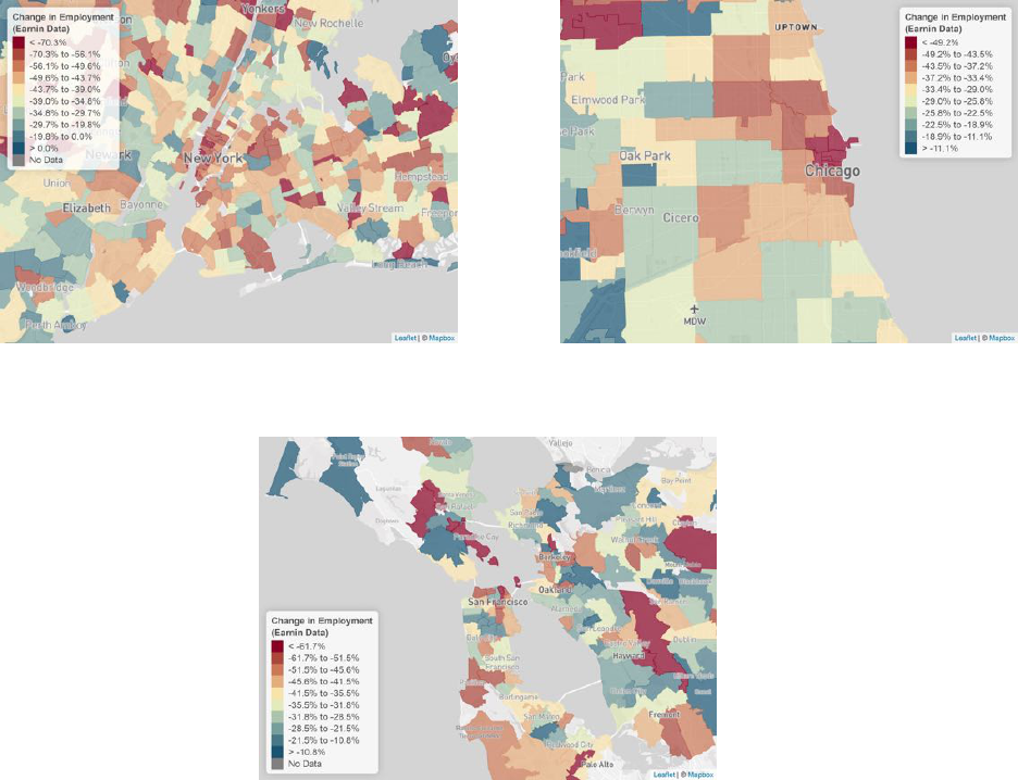
FIGURE 7: Changes in Employment Rates by ZIP Code

A. New York B. Chicago

C. San Francisco

Notes: This ﬁgure replicates Figure 4 using changes in employment at small businesses based on data from Earnin. The

change in employment is deﬁned as the average decrease inemployment at the ZCTA level from the period of January 8th to

March 10th, 2020 to the period of April 8th to April 28th, 2020. Data sources: Earnin, HomeBase

FIGURE 8: Changes in Employment and Job Postings vs. Rent

A. Hours Worked at Small Businesses and ZIP Median Rent

(Homebase)













    



B. Employment at Small Businesses and ZIP Median Rent (Earnin)















    



 

C. Job Postings for Low-Education Workers and County Median

Rent (Burning Glass)











   



D. Job Postings for High-Education Workers and County Median

Rent (Burning Glass)











   



Notes: This ﬁgure shows binned scatterplots of the relationship between median rent and both employment and job

postings. Binned scatter plots are constructed as indicated in Figure

3 by binning areas based on their median rent into 20

equally sized bins and computing the mean change in the outcome variable within each bin. Panels A presents the binned

scatter plots of the relationship between the average change in hours worked at businesses in the Homebase data between

January and April and median 2 bedro om rent at the ZCTA level using data from the. Panel B presents a similar binned

scatter plot showing the relationship between employment changes in the Earnin data and median 2 bedroom rent at the

ZCTA level. Both panels measure the percentage change from January 8-28th, 2020 to April 8-28th, 2020. The change in

hours worked in Panel A is constructed using Data from Homebase, which is comprised of small businesses. The change in

hours worked in Panel B is constructed using data from Earnin, and is shown separately for businesses above vs. below the

8th decile of ﬁrm size in the Earnin data. Panel C presents a binned scatterplot of the relationship between the percentage

change in job postings for workers with minimal or some education and median 2 bedroom rent (from the 2014-2018 ACS)

at the county level. Panel D presents a binned scatterplot of the relationship between percentage change in job postings for

workers with moderate, considerable or extensive education and median 2 bedro om rent, with a lowess ﬁt. Data sources:

Burning Glass, Earnin, Homebase

FIGURE 9: Geography of Unemployment in the Great Recession vs. COVID Recession





























   



Notes: This ﬁgure displays the share of job losses occurring in counties with diﬀering median incomes, for both the Great

Recession and the COVID recession. To construct the ﬁrst set of four bars, we ﬁrst calculate national employment loss between

2007 and 2010 using data from the BLS. We then group counties by median income, and compute the share of employment

loss that occurred in counties in each quartile of the distribution of county median income. The second set of bars replicates

the ﬁrst set of bars using total job losses that occurred between February 2020 and April 2020. The third set of bars reports

the allocation of county-level UI claims summed between March 15 and May 2 across counties in diﬀerent income quartiles.

In the ﬁrst set of bars, county median income is calculated using the 2006 ACS; in the second and third sets of bars, county

median income is calculated using the 2014-2018 ACS.

FIGURE 10: Changes in Consumer Spending vs. Workplace Rent for Low-Income Households

A. Change in Hours Worked vs Workplace Rent among Low-Income Households















      



B. Change in Spending vs Workplace Rent among Low-Income Households















      



Notes: This ﬁgure plots changes in hours worked (Panel A) or in consumer spending (Panel B) by ZCTA vs. the average

median 2 b edroom rent in the workplace ZIPs of individuals who live in a given ZCTA, restricting to ZCTAs in the bottom

quartile of the household income distribution. We construct the average median 2 bedroom rent variable by combining data

on the matrix of home residence by workplace ZCTAs taken from Census’ LEHD Origin-Destination Employment Statistics

(LODES) with data on median rents from the 2014-2018 ACS. In particular, we assign median rents from the ACS to each

ZCTA of workplace in the LODES data and then collapse workplace rents to each home ZCTA, weighting by the number of

jobs in each workplace ZCTA. In Panel A, the change in employment variable is based on data from Earnin. The change is

computed from Jan 5th to March 7th 2020 to the period of April 8th 2020 - April 28th 2020. In Panel B, the spending change

variable is based on data from Aﬃnity Solutions on total card spending, and the change is computed from the period of Jan

5th to March 7th 2020 to the period of March 22th 2020 - April 20nd 2020. Data sources: Aﬃnity Solutions, Earnin.

FIGURE 11: Causal Eﬀects of Re-Openings on Economic Activity: Event Studies

A. Case Study on Business Re-Openings: Colorado vs New Mexico































         

 



B. Re-Opened States vs. Control States: Consumer Spending















      



 



C. Re-Opened States vs. Control States: Employment















      



 



Notes: Panels A and B show seasonally-adjusted percent change in consumer spending in the Aﬃnity Solutions data (see

Section 2.1 for more details about the seasonal adjustment). Panel A shows the series for both New Mexico and Colorado;

Colorado partially reopened non-essential businesses on May 1, while New Mexico did not do so until May 16. Panel B

presents an event study of states that partially reopened non-essential businesses between April 20th and May 4th, compared

to a matched control group. We construct the control group separately for states on each opening day and then stack the

resulting event studies to align the events. Panel C replicates Panel B but instead plotting the percent change in employment

of workers using Earnin data. In Panels B-C, we provide the coeﬃcient from a diﬀerence-in-diﬀerence comparing treated vs.

untreated states in the two weeks following and the two weeks prior to the partial re-opening. Data sources: Aﬃnity Solutions,

Earnin

FIGURE 12: Impact of Stimulus Payments on Consumer Spending

A. Seasonally Adjusted Spending Changes by Income Quartile

-40%

-30%

-20%

-10%

Seasonally Adj. Pct. Change in Spending

Jan 7 Jan 21 Feb 4 Feb 18 Mar 3 Mar 17 Mar 31 Apr 14 Apr 28 May 12 May 26 Jun 9

Q1 ZCTA Income

Q4 ZCTA Income

Q1 Apr 7-13: -28.1%

Q4 Apr 7-13: -36.3%

Q4 Apr 15-21: -29.8%

Q1 Apr 15-21: -10.3%

B. Regression Discontinuity Plot for Lowest Income Quartile ZCTAs

-50%

-40%

-30%

-20%

-10%

10%

20%

Pct. Change in Spending Relative to Jan.

Apr 1 Apr 8 Apr 15 Apr 22 Apr 29

RD Estimate: 0.26 (0.07)

C. Regression Discontinuity Plot for Highest Income Quartile ZCTAs

-50%

-40%

-30%

-20%

-10%

10%

20%

Pct. Change in Spending Relative to Jan.

Apr 1 Apr 8 Apr 15 Apr 22 Apr 29

RD Estimate: 0.09 (0.04)

D. Regression Discontinuity Plot for Durable Goods

-30%

-20%

-10%

10%

20%

30%

Pct. Change in Spending Relative to Jan.

Apr 1 Apr 8 Apr 15 Apr 22 Apr 29

RD Estimate: 0.21 (0.06)

E. Regression Discontinuity Plot for In-Person Services

-90%

-80%

-70%

-60%

-50%

-40%

-30%

Pct. Change in Spending Relative to Jan.

Apr 1 Apr 8 Apr 15 Apr 22 Apr 29

RD Estimate: 0.07 (0.04)

Notes: This ﬁgure studies the eﬀect of the stimulus payments on spending in the Aﬃnity Solutions data. Panel A plots the

percent change in seasonally-adjusted consumer spending for both the lowest and highest population-weighted ZCTA median

household income quartiles. We use the ZCTA population and median household income estimates in the 2014-2018 ACS.

For panels B-D, each point is the national level of spending on that day divided by the average level of spending in January.

The points are residualised by day of week and ﬁrst of the month ﬁxed eﬀects. We estimate the ﬁxed eﬀects using data from

January 1, 2019, to May 10, 2019. The hollow-point and dashed line correspond to April 14th, which is excluded from the

regression. Panel B restricts to ZCTAs in the lowest income quartile. Panel C restricts to ZCTAs in the highest income

quartile. Panel D restricts to spending on durable goods as deﬁned in the notes for Figure 2. Panel E restricts to spending on

in-p erson services as deﬁned in the notes for Figure 2. Data source: Aﬃnity Solutions

FIGURE 13: Impact of Stimulus Payments on Business Revenue and Employment

A. Regression Discontinuity Plot for Lowest Rent Quartile ZCTAs

-60%

-50%

-40%

-30%

-20%

-10%

10%

Pct. Change in Revenue Relative to Jan.

Apr 1 Apr 8 Apr 15 Apr 22 Apr 29

RD Estimate: 0.18 (0.10)

B. Regression Discontinuity Plot for Highest Rent Quartile ZCTAs

-60%

-50%

-40%

-30%

-20%

-10%

10%

Pct. Change in Revenue Relative to Jan.

Apr 1 Apr 8 Apr 15 Apr 22 Apr 29

RD Estimate: 0.01 (0.06)

C. Revenue and Worker Earnings Changes Among Small

Businesses, by ZCTA Rent Quartile





















       



 

 

Notes: Panels A and B of this ﬁgure study the eﬀect of the stimulus payments on small business revenue in the Womply data.

In these panels, each point is the level of spending (in that ZCTA median 2-bedroom rent quartile) on that day divided by

the average level of spending in January. The points are residualised by day of week and ﬁrst of the month ﬁxed eﬀects. We

estimate the ﬁxed eﬀects using data from January 1, 2019, to May 10, 2019. The hollow-point and dashed line correspond

to April 14th, which is excluded from the regression. Panel C plots the percent change in the seven-day moving average of

small-business revenue using the Womply data and change in employment among Earnin users by ZCTA rent-quartile and

restricts to small businesses in the Earnin sample, as deﬁned by being in the bottom seven deciles of employer size. The

revenue series is seasonally-adjusted and the employment change series is relative to January 2020. Data sources: Earnin,

Womply

FIGURE 14: Impact of Paycheck Protection Program on Hours Worked

A. Change in Total Earnings by Decile of Firm Size, All Industries

Excl. NAICS 72

















        











B. Change in Total Earnings vs Decile of Firm Size, All Industries

Excl. NAICS 72















    



C. Change in Total Earnings by Firm Size and Employer ZCTA Rent

Quartile

















        











Notes: Panels A-C show the change in total earnings in a rep eated cross-section of Earnin users, by decile of employer size.

Each panel excludes workers in the Accommodation and Food Services sector (NAICS 72). The percent change for each week

is computed with respect to the average earnings between January 29th and February 25th. We estimate the size of ﬁrm

deciles 3-8 by matching Earnin employer names and locations to employer names and locations in ReferenceUSA data. We

estimate the size of ﬁrm deciles 1-2 by rescaling the number of Earnin users to total number of employees to match the national

distribution of ﬁrm sizes using data from the Statistics of U.S. Business (SUSB). The grey dashed line corresponds to April

3, 2020, the ﬁrst day for enrollment in the Paycheck Protection Program (PPP). Panels A and BC are both reweighted so

that industry composition is constant across ﬁrm size deciles. The change in earnings is ﬁrst calculated within each two-digit

NAICS code, and then reweighted so that the composition of industries within each decile of ﬁrm size matches the composition

of industries within all deciles plotted. Panel B plots the average percent change in earnings between April 8th and May 5th

against the median ﬁrm size in each decile. As NAICS code is not observed for ﬁrms in deciles 1-2 of Earnin data, the change

in earnings for deciles 1-2 reﬂects the change in earnings in all industries pooled, whereas the change in earnings for deciles

3-8 reﬂects the change in earnings in all industries other than Accommodation and Food Services. Panel C restricts to ﬁrms

that are eligible for the PPP (the 3rd and 4th deciles of employer size) and those that are ineligible (the 6th decile of employer

size) for the PPP, separately by rent quartile of work ZCTA. The population-weighted ZCTA rent income quartiles were

constructed using 2014-2018 ACS estimates of population and median-household income. Data source: Earnin

FIGURE 15: Eﬀects of COVID on Educational Progress by Income Group













         









Notes: We construct this series using data from Zearn Inc. at the class-week level, which we aggregate to the national-week-

income level according to the median household income of the Zip co des of Zearn schools (weighting by the average number

of students using the platform at each school during the base period). The key outcome is student progress, deﬁned as the

number of accomplishment badges earned in Zearn in each week, relative to the base period of January 6th-February 7th. Our

sample includes all classes with more than 10 students using Zearn during the base period, excluding those with fewer than

ﬁve users in all weeks. We index student progress to pre-COVID student progress by dividing weekly progress at the school

level by average weekly progress during the base period and then subtracting 1 to center the data around 0% change. Data

source: Zearn Inc.

APPENDIX FIGURE 1: Industry Shares of Consumer Spending and Business Revenues Across

Datasets

A. Compared to QSS

Percent of Total Service Revenue (%)

Finance

Health Care

Professional Services

Information

Admin Support

Transportation

Real Estate

Utilities

Other Services

Arts and Entertainment

Accomodation

Educational Services

QSS

Afﬁnity

Womply

B. Compared to MRTS

Percent of Total Retail and Food Service (%)

Motor Vehicles

Nonstore Retailers

Food & Beverage

Food Service

General Merchandise

Gas Stations

Health & Personal Care

Building Material

Clothing

Miscellaneous

Furniture

Electronics

Sporting & Hobby

MRTS

Afﬁnity

Womply

Notes: Panel A shows the NAICS two-digit industry mix for two private business credit card transaction datasets compared

with the Quarterly Services Survey (QSS), a survey dataset providing timely estimates of revenue and expenses for selected

service industries. Subsetting to the industries in the QSS, each bar represents the share of revenue in the speciﬁed sector

during Q1 2020. We construct spending and revenue shares for the private datasets, Aﬃnity and Womply, by aggregating

ﬁrm revenue (from card transactions) in January through March of 2020. Panel B shows the NAICS three-digit industry mix

for the same two private datasets compared with the Monthly Retail Trade Survey (MRTS), another survey dataset which

provides current estimates of sales at retail and food services stores across the United States. Subsetting to the industries in

the MRTS, each bar represents the share of revenue in the speciﬁed sector during January 2020. We construct revenue shares

for the private datasets, Aﬃnity and Womply, by aggregating ﬁrm revenue (from card transactions) in January 2020. Data

sources: Aﬃnity Solutions, Womply

APPENDIX FIGURE 2: Industry Shares of Employment Across Datasets































































Notes: This ﬁgure shows the NAICS two-digit industry mix for two private employment-based datasets compared with the

Quarterly Census of Employment and Wages (QCEW), an administrative dataset covering the near-universe of ﬁrms in the

United States. Each bar represents the share of employees in the given dataset who work in the speciﬁed sector. We construct

data for all establishments and small establishments using employment data from the Q1 2019 QCEW. Small establishments are

deﬁned as having fewer than 50 employees. We construct employment shares for the private datasets, Earnin and Homebase,

using January 2020 employment. We deﬁne employment in Earnin as the total number of worker-days in the month. We

deﬁne employment in Homebase as the number of unique individuals working a positive number of hours in the month. Data

sources: Earnin, HomeBase

APPENDIX FIGURE 3: Industry Shares of Job Postings in Burning Glass and Job Openings in

JOLTS















































 

Notes: This Figure displays the NAICS two-digit industry mix of job postings in Burning Glass and job openings in JOLTS,

the Job Openings and Labor Turnover Survey data provided by the U.S. Bureau of Labor Statistics, in January 2020. Data

source: Burning Glass

APPENDIX FIGURE 4: Spending Changes by Sector and Income Quartile







































 

 

Notes: This ﬁgure displays the change in spending by sector for the four quartiles of ZCTA median household income

(constructed using 2014-2018 ACS population and income estimates). These sectors were constructed by grouping together

similar merchant category codes, not all merchant category codes were used in this plot. The change in spending displayed

is (the log diﬀerence-in-diﬀerence of spending -1)*100, where the pre-period used is January 8th-28th and the post-period is

March 25th-April 14th. Data source: Aﬃnity Solutions

APPENDIX FIGURE 5: Spending Changes vs COVID Cases, by County

-28

-26

-24

-22

-20

Change in Consumer Spending (%)

Relative to Pre-COVID 2020

5 20 150 1100

County-level COVID-19 Cases Per 100,000 People (Log Scale)

Notes: To construct this ﬁgure, we divide the log COVID cases into 20 bins, each of which contain 5% of the population, and

plot the mean value of the log of COVID cases and change of spending variables within each bin, controlling for s tate ﬁxed

eﬀects and median-household income. COVID cases and decline in spending are both measured during the two week p eriod of

April 1st to April14th, and is benchmarked to the pre-period of January 8th to January 28th. Data source: Aﬃnity Solutions

APPENDIX FIGURE 6: Small Business Revenue Changes vs. Local Income Distribution

A. Retail Services (Excluding Auto and Gas)















        







B. Food Services and Accommodations



















Notes: This ﬁgure compares weekly total consumer spending (from Aﬃnity Solutions purchase data) and small business

revenue (from Womply) normalized to the average pre-COVID levels of each year. The pre-COVID period is deﬁned as

January 8 - March 10 and we normalize within each calendar year to account for year ﬁxed eﬀects. Following the sectors

deﬁned in the Monthly Retail Trade Survey (MRTS), Panel A restricts to speciﬁcally retail trade sectors (NAICS code 44-45)

excluding motor vehicles (NAICS code 441) and gas (NAICS code 447), and Panel B restricts speciﬁcally to food services and

accommodations (NAICS code 72). Data sources: Aﬃnity Solutions, Womply

APPENDIX FIGURE 7: Changes in Small Business Revenues by ZIP Code for Food and

Accommodation Service Businesses

A. New York City B. Chicago

C. San Francisco

Notes: This Figure displays ZCTA-level maps of the MSAs corresponding to New York City, San Francisco, and Chicago,

colored by their respective deciles of Womply change in revenue for small businesses classiﬁed as NAICS 72 within each MSA.

This ﬁgure corresponds to the process described in the notes for Figure 4. Data source: Womply

APPENDIX FIGURE 8: Changes in Small Business Revenues by County

Notes: This ﬁgure replicates Figure 4 but for the entire United States instead of a single city and its surrounding area and

graphing counties instead of ZCTAs. See notes to Figure 4 for details. Data source: Womply

APPENDIX FIGURE 9: Womply Business Revenue vs. Poverty Share, Top 1% Share, and Gini

by County

A. Gini Index

















   



B. Share of Population in Top 1% of Income Distribution

















     



C. Share of Population below Poverty Line

















    



Notes: This Figure replicates Figure 5 but compares the declines with diﬀerent measures of inequality. Panel A compares the

within county Gini index against the declines. Panel B uses the share of the county with incomes at the top 1% of the income

distribution. Panel C compares the declines with the share of the county population with incomes below the poverty line in

the 2010 decennial census. See notes to Figure 5 for details. Data source: Womply

APPENDIX FIGURE 10: Womply Business Closures vs. Rent by ZIP

















   



Notes: This ﬁgure replicates Panel C of Figure 5 but shows average changes in small businesses that remain open

instead of changes in revenue. See notes to Figure 5 for details.

Data source: Womply

APPENDIX FIGURE 11: Changes in Wages, Hours Worked and Earnings Over Time

A. Earnin























       







B. HomeBase























       









Notes: This ﬁgure compares changes in mean wages and employment relative to January 2020 within the Earnin (Panel A)

and HomeBase (Panel B) datasets.We construct daily wages for both Earnin and HomeBase by calculating the mean wage on

each day. In the HomeBase dataset, we condition on workers being employed by restricting the sample to workers who are

observed working in every week of the series. We construct employment in the Earnin and Homebase data and earnings in the

Homebase data by summing the total number of hours worked in each day and the total wages earned in each day, respectively.

We then take the mean value of each series over the prior seven days and norm to the average value of the seven-day moving

average over the period January 4 - January 31, 2020.

Data sources: Earnin, HomeBase

APPENDIX FIGURE 12: Changes in Employment Rates by County

Notes: This ﬁgure replicates Figure 7 but for the entire United States instead of a single city and its surrounding area. See

notes to Figure 7 for details. Data sources: Earnin

APPENDIX FIGURE 13: Changes in Total Employment by Firm Size









         



Notes: This ﬁgure displays the average declines in employment among workers in the Earnin data, separately for each ﬁrm size

decile. The decline is calculated by taking total employment at the ﬁrm decile level in a pre-period that spans from January

8th, 2020 to January 28th, 2020, and comparing to employment in a post-period that spans from April 1, 2020 to April 21,

2020. Firms are classiﬁed into ﬁrm size deciles based on total number of Earnin users at the ﬁrm. Data source: Earnin

APPENDIX FIGURE 14: Changes in Employment Rates by ZIP Code for Food and

Accommodation Service Businesses

A. New York City B. Chicago

C. San Francisco

Notes: This Figure displays ZCTA-level maps of the MSAs corresponding to New York City, San Francisco, and Chicago,

coloured by their respective deciles of change in hours worked in businesses classiﬁed as NAICS 72 within each MSA. We

calculate total hours worked in each ZCTA by summing total hours worked in Earnin data with total hours worked in

Homebase data, restricting to NAICS 72 employers in both datasets. We then calculate changes in hours worked in each

ZCTA as described in the notes to Figure 7. Data sources: Earnin, HomeBase

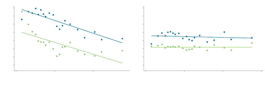
APPENDIX FIGURE 15: Changes in Job Postings vs. Rent Over Time

A. Job Postings for Low-Education Workers and County Median

Rent, Over Time























   



B. Job Postings for High-Education Workers and County Median

Rent, Over Time























   



Notes: This ﬁgure shows binned scatterplots of the relationship between median rent and changes in job postings between a

pre-period of January 8 - March 10 and the periods March 25 - April 14 or the period May 30-June 5. The change in job

postings is computed using Burning Glass data. Median two-bedroom rent is computed using the 2014-2018 ACS at the county

level. Panel C presents a binned scatterplot of the relationship between the percentage change in job postings for workers with

minimal or some education and median 2 bedroom rent. Panel D presents a binned scatterplot of the relationship between

the percentage change in job postings for workers with moderate, considerable or extensive education and median 2 bedroom

rent. Data source: Burning Glass

APPENDIX FIGURE 16: Legislated Stay-at-Home Orders and Non-Essential Business Closures























     

  



Notes: This ﬁgure shows percent change in seasonally-adjusted consumer spending in the Aﬃnity Solutions data, pooling

together states that closed non-essential business early (between March 19th and March 24th), states that closed non-essential

businesses late (between March 30th and April 6th), and those that never closed. Data source: Aﬃnity Solutions

APPENDIX FIGURE 17: IRS Transactions Among Earnin Users











     

Notes: This ﬁgure displays the total dollar amount of IRS transactions for Earnin users. Data source: Earnin

APPENDIX FIGURE 18: Impact of Stimulus on the Composition of Consumer Spending

25%

50%

75%

100%

January

Pre-Stimulus

Post-Stimulus

Composition of Recovery

Remote Services

21%

Durable Goods

23%

Non-Durable Goods

23%

In-person Services

32%

Remote Services

24%

Durable Goods

29%

Non-Durable Goods

29%

In-person Services

18%

Remote Services

23%

Durable Goods

30%

Non-Durable Goods

27%

In-person Services

20%

Remote Services

19%

Durable Goods

44%

Non-Durable Goods

19%

In-person Services

18%

Composition of Spending

Notes: See notes of Figure 2 Panel B. The pre-stimulus, post-COVID period is deﬁned as March 25th-April 14th. The

post-stimulus period is deﬁned as April 29th to May 5th. The total recovery is computed use the post-stimulus period

and the average weekly spending in the pre-stimulus period. This ﬁgure disaggregates spending by Merchant Category

Codes (MCCs), grouping together similar MCCs.We deﬁne durable goods as the following MCC groups: motor vehicles,

sporting goods and hobby, home improvement centers, consumer electronics, and telecommunications equipment. Non-durable

goods include wholesale trade, agriculture, forestry and hunting, general merchandise, apparel and accessories, health and

personal care stores, and grocery stores. Remote services include utilities, professional/scientiﬁc services, public administration,

administration and waste services, information, construction, education, and ﬁnance and insurance. In-person services include

real estate and leasing, recreation, health care services, transportation and warehousing services, and accommodation and

food, as well as barber shops, spas, and assorted other services. Data source: Aﬃnity Solutions

APPENDIX FIGURE 19: Histograms of PPP Eligibility Firm Size Cutoﬀs for Firms with 300 to

700 Employees

A. Eligibility Cutoffs in Reference USA Data















    



B. Eligibility Cutoffs in Earnin Data















    



C. Share of Earnin Firms With Over 500 Employees, By Earnin Decile













       



Notes: This ﬁgure plots a histogram of the ﬁrm size cutoﬀs for PPP eligibility in the set of ﬁrms in Reference USA and the

set of ﬁrms in the Earnin sample. In the reference USA data, we take the establishment-size-weighted distribution of PPP

employee-based eligibility thresholds, which are based on parent company size (except in the case of NAICS 72, which is not

included here). In the Earnin sample, we assign a ﬁrm size threshold for which the individual’s ﬁrm would be eligible for PPP

loans. Panel C shows the proportion of ﬁrms in the Earnin data whose parent company has more than 500 employees, split

by ﬁrm size deciles based on number of Earnin users.

APPENDIX FIGURE 20: Impact of Paycheck Protection Program on NAICS 72













        











Notes: This ﬁgure replicates Figure 14a for NAICS 72. See notes for Figure 14. Data source: Earnin