
JAIPUR ENGINEERING COLLEGE AND RESEARCH CENTRE
JECRC Campus, Shri Ram Ki Nangal, Via-Vatika, Jaipur
LAB MANUAL
Lab : Heat Transfer Lab
Lab Code : 5ME4-22
Branch : Mechanical Engineering
Year : 3
rd
Year
Department of Mechanical Engineering
Jaipur Engineering College and Research Centre, Jaipur
(RTU, Kota)

JAIPUR ENGINEERING COLLEGE AND RESEARCH CENTRE
JECRC Campus, Shri Ram Ki Nangal, Via-Vatika, Jaipur
INDEX
S.NO
CONTENTS
PAGE
NO.
1
VISION/MISION
3
2
PROGRAM EDUCATIONAL OBJECTIVES (PEOs)
4
3
PROGRAM OUTCOMES (POs)
5
4
COURSE OUTCOMES (COs)
6
5
MAPPING OF COs with POs
7
6
SYLLABUS
8
7
BOOKS
9
8
INSTRUCTIONAL METHODS
10
9
LEARNING MATERIALS
11
10
ASSESSMENT OF OUTCOMES
12
11
INSTRUCTIONS SHEET
13
Exp:- 1
Objective: To Determine Thermal Conductivity of Insulating
Powders
14
Exp:- 2
Objective :To Determine Thermal Conductivity of a Good Conductor
of Heat (Metal Rod)
19
Exp:-3
Objective :To determine the transfer Rate and Temperature
Distribution for a Pin Fin
25
Exp:-4
Objective :To Measure the Emissivity of the Test plate Surface
30
Exp:-5
Objective: To Determine Stefan Boltzmann Constant of Radiation
Heat Transfer.
34
Exp:-6
Objective :To Determine the Surface Heat Transfer Coefficient For
Heated Vertical Cylinder in Natural Convection
39
Exp:-7
Objective :Determination of Heat Transfer Coefficient in Drop Wise
and Film Wise condensation
44
Exp:-8
Objective :To Determine Critical Heat Flux in Saturated Pool Boiling
48
Exp:-9
Objective :To Study and Compare LMTD and Effectiveness in
Parallel and Counter Flow Heat Exchangers
51
Exp:-10
Objective :To Find the Heat transfer Coefficient in Forced
Convection in a tube.
54
Exp:-11
Objective : To study the rates of heat transfer for different materials
and geometries.
58

JAIPUR ENGINEERING COLLEGE AND RESEARCH CENTRE
JECRC Campus, Shri Ram Ki Nangal, Via-Vatika, Jaipur
Exp:-12
Objective : To understand the importance and validity of engineering
assumptions through the lumped heat capacity method
63
1. VISION & MISSION
VISION:
➢ The Mechanical Engineering Department strives to be recognized globally for
outcome based technical knowledge and to produce quality human resource, who can
manage the advance technologies and contribute to society
MISSION:
➢ To impart quality technical knowledge to the learners to make them globally
competitive mechanical engineers.
➢ To provide the learners ethical guidelines along with excellent academic environment
for a long productive career
➢ To promote industry-institute relationship

JAIPUR ENGINEERING COLLEGE AND RESEARCH CENTRE
JECRC Campus, Shri Ram Ki Nangal, Via-Vatika, Jaipur
2. PROGRAM EDUCATIONAL OBJECTIVES
PEO1: To provide students with the fundamentals of engineering sciences with more
emphasis in Mechanical Engineering by way of analysing and exploiting engineering
challenges.
PEO2: To train students with good scientific and engineering knowledge so as to
comprehend, analyse, design, and create novel products and solutions for the real life
problems in Mechanical Engineering.
PEO3: To inculcate professional and ethical attitude, effective communication skills,
teamwork skills, multidisciplinary approach, entrepreneurial thinking and an ability to
relate Mechanical Engineering issues with social issues.
PEO4: To provide students with an academic environment aware of excellence,
leadership, written ethical codes and guidelines, and the self-motivated life-long
learning needed for a successful professional career in Mechanical Engineering.
PEO5: To prepare students to excel in industry and higher education by educating
students along with high moral values and knowledge in Mechanical Engineering.

JAIPUR ENGINEERING COLLEGE AND RESEARCH CENTRE
JECRC Campus, Shri Ram Ki Nangal, Via-Vatika, Jaipur
3. PROGRAM OUTCOMES
1. Engineering knowledge: Apply the knowledge of mathematics, science, engineering
fundamentals, and an engineering specialization to the solution of complex
engineering problems.
2. Problem analysis: Identify, formulate, research literature, and analyze complex
engineering problems reaching substantiated conclusions using first principles of
mathematics, natural sciences, and engineering sciences.
3. Design/development of solutions: Design solutions for complex engineering problems
and design system components or processes that meet the specified needs with
appropriate consideration for the public health and safety, and the cultural, societal,
and environmental considerations.
4. Conduct investigations of complex problems: Use research-based knowledge and
research methods including design of experiments, analysis and interpretation of data,
and synthesis of the information to provide valid conclusions.
5. Modern tool usage: Create, select, and apply appropriate techniques, resources, and
modern engineering and IT tools including prediction and modeling to complex
engineering activities with an understanding of the limitations.
6. The engineer and society: Apply reasoning informed by the contextual knowledge to
assess societal, health, safety, legal and cultural issues and the consequent
responsibilities relevant to the professional engineering practice.
7. Environment and sustainability: Understand the impact of the professional
engineering solutions in societal and environmental contexts, and demonstrate the
knowledge of, and need for sustainable development.
8. Ethics: Apply ethical principles and commit to professional ethics and responsibilities
and norms of the engineering practice.
9. Individual and team work: Function effectively as an individual, and as a member or
leader in diverse teams, and in multidisciplinary settings.
10. Communication: Communicate effectively on complex engineering activities with the
engineering community and with society at large, such as, being able to comprehend
and write effective reports and design documentation, make effective presentations,
and give and receive clear instructions.
11. Project management and finance: Demonstrate knowledge and understanding of the
engineering and management principles and apply these to one’s own work, as a
member and leader in a team, to manage projects and in multidisciplinary
environments.
12. Life-long learning: Recognize the need for, and have the preparation and ability to
engage in independent and life-long learning in the broadest context of technological
change.

JAIPUR ENGINEERING COLLEGE AND RESEARCH CENTRE
JECRC Campus, Shri Ram Ki Nangal, Via-Vatika, Jaipur
4. COURSE OUTCOMES
HEAT TRANSFER [5ME7A]
Class: Sem.: 5
th
SEM B.Tech. Branch: Mechanical Engineering
Schedule per Week Practical Hrs.: 2 Hrs Examination Time = 2 Hours
Maximum Marks = [Sessional/Mid-term (30 ) & End-term ( 20)]
On successful completion of this course the students will be able to:
1. To analyze the conduction and convection processes that occurs in multiple aspects of
daily life.
2. To examine the process of radiation and relate its properties to design of thermal
systems.

JAIPUR ENGINEERING COLLEGE AND RESEARCH CENTRE
JECRC Campus, Shri Ram Ki Nangal, Via-Vatika, Jaipur
5. MAPPING OF COs with POs
COURSE
OUTCOMES
PROGRAM OUTCOMES
1
2
3
4
5
6
7
8
9
10
11
12
I
3
1
1
1
0
1
2
0
2
1
0
3
II
3
2
2
1
1
1
2
0
2
1
1
3

JAIPUR ENGINEERING COLLEGE AND RESEARCH CENTRE
JECRC Campus, Shri Ram Ki Nangal, Via-Vatika, Jaipur
6. SYLLABUS
HEAT TRANSFER LAB [5ME4-22]
Class: Sem. 5
th
SEM
Evaluation
Branch: ME
Schedule per week
Practical Hrs: (2)
Examination Time=Two ( 02) Hours
Maximum Marks = 50
[Sessional/Mid-term (30) & End-term(20)
S.N.
NAME OF EXPERIMENT
1
To Determine Thermal Conductivity of Insulating Powders
2
To Determine Thermal Conductivity of a Good Conductor of Heat (Metal Rod)
3
To determine the transfer Rate and Temperature Distribution for a Pin Fin
4
To Measure the Emissivity of the Test plate Surface
5
To Determine Stefan Boltzmann Constant of Radiation Heat Transfer.
6
To Determine the Surface Heat Transfer Coefficient For Heated Vertical
Cylinder in Natural Convection
7
Determination of Heat Transfer Coefficient in Drop Wise and Film Wise
condensation
8
To Determine Critical Heat Flux in Saturated Pool Boiling
9
To Study and Compare LMTD and Effectiveness in Parallel and Counter Flow
Heat Exchangers
10
To Find the Heat transfer Coefficient in Forced Convection in a tube.
11
To study the rates of heat transfer for different materials and geometries
12
To understand the importance and validity of engineering assumptions
through the lumped heat capacity method.

JAIPUR ENGINEERING COLLEGE AND RESEARCH CENTRE
JECRC Campus, Shri Ram Ki Nangal, Via-Vatika, Jaipur
7. BOOKS
1. Text book of Heat and mass transfer by D.S. Kumar, S.K. Kataria and Sons (2009)
2. J.P.Holman, Heat and Mass Transfer, TMH
3. Yunus Cenegal, HMT-Practical Approach, TMH.
3. M.M.Rathore, Engineering Heat and Mass Transfer, University Science Press
8. INSTRUCTIONAL METHODS
8.1. Direct Instructions:
I. Black board presentation.
II. Power point presentation.
8.2. Interactive Instruction:
I. Practical on respective equipment.
II. Practical Examples.
8.3. Indirect Instructions:
I. Problem solving
9. LEARNING MATERIALS
9.1. Lab Manual
9.2. Reference Books
10. ASSESSMENT OF OUTCOMES
10.1. End term Practical exam (Conducted by RTU, KOTA)
10.2. Quiz
10.3. Daily Lab interaction.

JAIPUR ENGINEERING COLLEGE AND RESEARCH CENTRE
JECRC Campus, Shri Ram Ki Nangal, Via-Vatika, Jaipur
11. INSTRUCTIONS SHEET
We need your full support and cooperation for smooth functioning of the lab.
DO’s
1. Please switch off the Mobile/Cell phone before entering lab.
2. Enter the lab with proper manual write-up and necessary writing instruments.
3. Check whether all peripheral are available at your experimental set-up before
starting the experiment.
4. Intimate the lab incharge whenever you are incompatible in using the
instrument.
5. Arrange all the peripheral and seats before leaving the lab.
6. Properly switch-off the instrument before leaving the lab.
7. Keep the bag outside in the racks.
8. Enter the lab on time and leave at proper time.
9. Maintain the decorum of the lab.
10. Utilize lab hours in the corresponding experiment.
DON’TS
1. No one is allowed to bring storage devices like Pan Drive /Floppy etc. in the
lab.
2. Don’t mishandle the instrument in the lab.
3. Don’t bring any external material in the lab.
4. Don’t make noise in the lab.
5. Don’t bring the mobile in the lab. If extremely necessary then keep ringers off.
6. Don’t enter in the lab without permission of lab Incharge.
7. Don’t litter in the lab.
8. Don’t misplace any experiment measuring instrument.
9. Don’t carry any lab equipments outside the lab.
BEFORE ENTERING IN THE LAB
1. All the students are supposed to prepare the theory regarding the next experiment
2. Students are supposed to bring the practical file and the lab copy.
3. Previous practical should be written in the practical file.
4. Any student not following these instructions will be denied entry in the lab.
WHILE WORKING IN THE LAB
1. Adhere to experimental schedule as instructed by the lab incharge.
2. Get the previously executed experiment signed by the instructor.
3. Get the output of the current experiment checked by the instructor in the lab copy.

JAIPUR ENGINEERING COLLEGE AND RESEARCH CENTRE
JECRC Campus, Shri Ram Ki Nangal, Via-Vatika, Jaipur
4. Each student should perform the experiment with your group members at each turn of
the lab.
5. Take responsibility of valuable accessories.
6. Concentrate on the assigned practical and do not play games.
7. If anyone caught red handed carrying any equipment of the lab, then he will have to
face serious consequences.

JAIPUR ENGINEERING COLLEGE AND RESEARCH CENTRE
JECRC Campus, Shri Ram Ki Nangal, Via-Vatika, Jaipur
Thermal Conductivity of Insulating Powder
Experiment No. 1
OBJECTIVE:. To determine the thermal conductivity of Insulating Powders.
INTRODUCTION:
Knowledge of thermal properties like thermal conductivity of a powder is important for
computing heat transfer rates (losses) in many fields of engineering such as mechanical and
chemical. Determination of thermal conductivity of powders is bit different as powders are
generally porous and can exist at different void fraction depending upon pressure exerted on
it. The thermal conductivity of powder is determined by passing measured quantity of heat
through a known thickness of powder and monitoring the temperature difference. The
thermal conductivity, K of the powder is then computed by equation (i).
Q = -KA(Δt/x)……………………………………………………….(1)
Where, Q= the rate of heat transfer, KJ/s
A= area of heat transfer, m
2
Δt= temperature drop across the powder layer of thickness ‘x’,
o
C
x= thickness of powder layer, m
To apply equation (i) for determination of thermal conductivity, it is necessary that all the
heat is transported through conduction across the sample. The condition necessitates that the
thickness of powder layer be very small so that the conduction is across the layer.
APPARATUS:
The apparatus mainly consists of guarded hot plate assembly to measure thermal conductivity
of powder. The container in which, the assembly is kept well insulated using thermal
insulation, and the necessary instrumentation for measurement and control of voltage, current
and temperature. One top guard and second ring guard heaters are provided to stop heat
leaking from the main heater and whatever heat is generated in the main heater passes
through the powder layer and goes to the cooling chamber. In this way longitudinal transfer
of heat in conduction mode is ensured which qualifies the equation (i) to be used for the
computation of thermal conductivity.

JAIPUR ENGINEERING COLLEGE AND RESEARCH CENTRE
JECRC Campus, Shri Ram Ki Nangal, Via-Vatika, Jaipur
Thermal Conductivity of Insulating Powder
The apparatus is properly instrumented to measure voltage and current fed to main heater.
The wattage to different heaters is controlled by dimmer state. The temperatures at different
points are measured using copper constantan thermocouples and is displayed using a digital
temperature indicator with resolution of 0.1
o
c. Thermocouples are scanned manually using a
six point selector switch.
It is necessary that the guarded hot plate assembly by assembled every time when it is
required to find out the thermal conductivity of a new powder. The procedure for proper
assembly of the unit is detailed below.
EXPERIMENTAL PROCEDURE:
1. Assemble the apparatus as per the instructions given below.
2. Connect the thermocouples to the selector switch.
3. Connect the three heaters (main, top guard, ring guard) to the socket meant for
these.
4. Bring the three dimmer states (use to energize three heaters) to zero output state.
5. Switch ON the cooling water to flow the apparatus.
6. Switch ON the main switch and more the initial temperature of all the six
thermocouples.
7. Energize the main heater using the dimmer state to about 35 volts. The power
input to the main heater should be such that its hot surface gets the desired
temperature and a low temperature drop is achieved across the powder film.
8. Energize top guard and ring guard heaters using the dimmer states gradually so
that the temperature shown by thermocouples 5 to 6 are properly balanced.
9. Wait for steady state to reach and note down the temperatures of all the 6
thermocouples and voltage & current readings for main heater, ring and top guard
heater.
10. Step vii- ix is repeated for measuring thermal conductivity of powder at higher
mean temperature.
OBSERVATION TABLE:
Powder =
Diameter of main heater plate, m =
Powder space diameter, m =
Space thickness, x, m =

JAIPUR ENGINEERING COLLEGE AND RESEARCH CENTRE
JECRC Campus, Shri Ram Ki Nangal, Via-Vatika, Jaipur
Thermal Conductivity of Insulating Powder
CALCULATION:
Q = -KA(Δt/x)……………………………………………………….(1)
Where, Q= the rate of heat transfer, KJ/s
A= area of heat transfer, m
2
Δt= temperature drop across the powder layer of thickness ‘x’,
o
C
x= thickness of powder layer, m
PRECAUTIONS:
1. Do not increase voltage more than 55 volts.
2. Do not touch the surface of heating tube.
3. Do not touch the insulation bags.
4. The temperature of the three heaters i.e. main, top and ring must be nearly same.
5. The water should not be re-circulated.
APPLICATION:
Heater(s)
Voltage(V)
Current(I)
Wattage= VI
Main
Ring guard
Top guard
Location(s)
Thermocouple number and temperature,
o
c
Main heater
plate
1
2
Cold plate
3
4
Ring guard
5
Top guard
6

JAIPUR ENGINEERING COLLEGE AND RESEARCH CENTRE
JECRC Campus, Shri Ram Ki Nangal, Via-Vatika, Jaipur
Thermal Conductivity of Insulating Powder
Thermal conductivity is the property of a material which helps to know ability of a material
to conduct heat. By knowing the thermal conductivity of a material/powder one can decide
whether the material/powder is a good conductor of heat or not. So that the material/powder
can be used as conductor of heat or as insulator.
EXPECTED OUTCOME:
The Thermal conductivity of insulating powder is found to be about --------------
-- W/m
2
k
COMMENT BY STUDENT:
VIVA VOCE:
Q1- Define thermal conductivity.
Q2- What is a thermal resistance.
Q3-What is a thermal conductance.
Q4- Which type of powder is used to measure the thermal conductivity.
Q5-What is a thermocouples.
Q6-Explane the one dimension heat flow in metal road.
Q7-What is unit of thermal conductivity.
Q9-What is heat transfer coefficient.

JAIPUR ENGINEERING COLLEGE AND RESEARCH CENTRE
JECRC Campus, Shri Ram Ki Nangal, Via-Vatika, Jaipur
Thermal Conductivity of Metal Rod
Experiment No. 2
OBJECTIVE:. To determine the Thermal Conductivity of a good conductor of heat
(Metal Rod).
INTRODUCTION: Thermal conductivity of a substance is a physical property, defined as
the ability of a substance to conduct heat .Thermal conductivity of material depends on
chemical composition, state of matter, crystalline structure of a solid, the temperature,
pressure and whether or not it's a homogeneous material.The heater will heat the bar on its
end one and heat will be conducted through the bar at the other end. Since the rod is insulated
from outside,it can safely assume that the heat transfer along the copper rod is mainly due to
axial conduction and at steady state the heat conducted shall be equal to the heat absorbed by
water at cooling end. The heat conducted at steady state shall create a temperature profile
within the rod.
The steady state heat balance at the rear end of the end is:Heat absorbed by cooling water
Q=MCpdT
Heat conducted through the rod in axial direction:
Q=-KA(dT/dX)
At steady state,
Q=-KA(dT/)=MCpdT
So Thermal conductivity of rod may be expressed as,
K=(MCpdT)/(-A(dT/dX))
The assumption that at steady state, the heat flow is mainly due to axial conduction can be
verified by the reading of temperature sensor fixed in the. Insulation material around the rod

JAIPUR ENGINEERING COLLEGE AND RESEARCH CENTRE
JECRC Campus, Shri Ram Ki Nangal, Via-Vatika, Jaipur
Thermal Conductivity of Metal Rod
in the radial direction. Less variation in these reading shall confirm the assumption .The value
of dT/dX is obtained as the slope of graph between T vs X.
APPARATUS:
The apparatus consists of a metal bar ,one end of which is heated by a electric heater while
other end projects inside the cooling water jacket .The middle portion of bar is surrounded by
a cylindrical shell filled with the asbestos insulating powder .The temperature of bar is
measured at different section .The heater is provided with a thermostat for controlling the
heat input .Water under constant head condition is circulated through the jacket and its flow
rate and temperature rise are noted by two temperature sensors provided at inlet and outlet of
the water.
Electricity Supply: 1 phase, 220V AC,2 Amp, Water Supply, Drain, Table for set-up support
EXPERIMENTAL PROCEDURE:
1. Connect cold water supply at inlet of the cooling chamber.
2. Connect outlet of the cooling chamber to drain.
3. Ensure that all ON/OFF switches given on the panel are at OFF position.
4. Ensure that variac knob is at zero (0) position given on the panel.
5. Start water supply at constant head.
6. Now switch on the Main Power supply (220VA, 50 Hz).
7. Switch on the panel with the help of Main ON/OFF switch given on the panel
8. Fix the power input to the heater with the help of Variac, Voltmeter and Ammeter
provided.
9. After 30 Minute start recording the temperature of various point at each 5 Minutes
interval.
10. If temperature reading are same for three times, assume that the steady state is
achieved.
11. Record the final temperatures.
OBSERVATION TABLE:
Voltage - V volt, Current - I amp
S.No
T1
(◦C)
T2
(◦C)
T3
(◦C)
T4
(◦C)
T5
(◦C)
T6
(◦C)
T7
(◦C)
T8
(◦C)

JAIPUR ENGINEERING COLLEGE AND RESEARCH CENTRE
JECRC Campus, Shri Ram Ki Nangal, Via-Vatika, Jaipur
Thermal Conductivity of Metal Rod
CALCULATION:
K =MCp(∆T) / [-A{dT/dX}]
PRECAUTIONS:
1. Use the stabilize A.C. single phase supply only.
2. Never switch on the main power supply before ensuring that all the 0N/OFF switches
given on the panel are at OFF position.
3. Voltage to heater to be starts and increase slowly.
4. Keep all the assembly undisturbed.
5. Never run the apparatus if power supply is less than 180 volt and above than 240 volts.
6. Operate selector switch of temperature indicator gently.
7. Always keep the apparatus free from dust.
8. There is the possibility of getting abrupt result if the supply voltage is fluctuating or if he
satisf
APPLICATION:
Thermal conductivity is important in material science, research, electronics, building
insulation and related fields, especially where high operating temperatures are achieved. High
energy generation rates within electronics or turbines require the use of materials with high
thermal conductivity such as copper, aluminium, and silver. On the other hand, materials with
low thermal conductance, such as polystyrene and alumina, are used in
building construction or in furnaces in an effort to slow the flow of heat, i.e. for insulation
purposes.

JAIPUR ENGINEERING COLLEGE AND RESEARCH CENTRE
JECRC Campus, Shri Ram Ki Nangal, Via-Vatika, Jaipur
Thermal Conductivity of Metal Rod
EXPECTED OUTCOME: The Thermal conductivity of metal rod is found to
be about ---------------- W/m
2
k
COMMENT BY STUDENT:
VIVA VOCE:
1. Define thermal conductivity.
2. What type of thermocouples are used?
3. Explain the Fourier’s law?
4. Which type of heater is used in the experiment?
5. What material having higher thermal conductivity?

JAIPUR ENGINEERING COLLEGE AND RESEARCH CENTRE
JECRC Campus, Shri Ram Ki Nangal, Via-Vatika, Jaipur
Pin Fin
Experiment No. 3
OJECTIVE:. To determine the heat transfer rate and Temperature distribution for a Pin
Fin
INTRODUCTION:
Extended surfaces or fins are used to increase the heat transfer rate from a surface to a fluid
wherever it is not possible to increase the value of the surface heat transfer coefficient or the
temperature difference between the surface and the fluid. The use of this is very common and
they are fabricated in a variety of shapes circumferential fins around the cylinder of a
motorcycle engine and fins attached to condenser tubes of a refrigerator are few familiar
examples.
Natural convection phenomenon is due to the temperature difference between the surface and
the fluid and is not created by any external agency. Forced convection phenomenon is due to
the temperature difference between the surface and the fluid and is created by any external
agency, such as blower, pump etc. The experimental heat transfer coefficient is given for both
the free and forced convection.
h
exp
= Q
a
/ A
s
ΔT
Theoretical heat transfer coefficient for free and forced convection, can be calculated by
following formulae:
h
th
= N
u
K/D
Where h
exp
, h
th
are experimental and theoretical heat transfer coefficient respectively.
Q
a
is amount of heat transfer, A
s
is heat transfer area and ΔT is temperature difference.
Nu is Nusselt no., k is thermal conductivity and D is diameter. It is obvious that a fin surface
stick out from primary heat transfer surface. The temperature difference with surrounding
fluid will steadily diminish as one moves out along the fin. The design of the fins therefore
requires knowledge of the temperature distribution in the fin. The main object of this
experimental set up is to study the temperature distribution in a simple pin fin.
It consists of pin type fin fitted in a duct. A blower is provided on one side of duct. Air flow
rates can be varied by given flow control valve. A heater is provided to heats one end of fin
and heat flows to another end. Heat input to the heater is given through variac digital
voltmeter and digital ammeter are provided for heat measurement. Digital temperature
indicator measures temperature distribution along the fin. Airflow is measured with the help
of orifice meter and the water manometer fitted on the board.

JAIPUR ENGINEERING COLLEGE AND RESEARCH CENTRE
JECRC Campus, Shri Ram Ki Nangal, Via-Vatika, Jaipur
Pin Fin
Fin Parameter (m) is given a
Fin Effectiveness is given as
The temperature profile within a pin fin is given by:
=
=
EXPERIMENTAL PROCEDURE:
For FREE Convection
1. Ensure that mains ON/OFF switch given on the panel is at OFF position & dimmer
stat is at zero position.
2. Connect electtc supply to the set up.
3. Switch ON the mains ON / OFF switch.
4. Set the heater input by the dimmer stat, voltmeter in the range 40 to 100 V.
5. After 1.5 hrs. note down the reading of voltmeter, ampere meter and temperature
sensors at every 10 minutes interval
6. When experiment is over set the dimmer stat to zero position.
7. Switch OFF the mains ON/OFF switch.
8. Switch OFF electric supply to the set up.
For Forced Convection
1. Ensure that mains ON/OFF switch given on the panel is at OFF position & dimmer
stat is at zero Position.
2. Connect electric supply to the set up.
3. Fill water in manometer up to half of the scale, by opening PU pipe connection from
the air flow
4. Pipe and connect the pipe back to its position afler doing so.
5. Switch ON the mains ON / OFF switch.
6. Set the heater input by the dimmer stat, voltmeter in the range 40 to 100 V.
7. Switch ON the blower.
8. Set the flow of air by operating the valve V1.

JAIPUR ENGINEERING COLLEGE AND RESEARCH CENTRE
JECRC Campus, Shri Ram Ki Nangal, Via-Vatika, Jaipur
Pin Fin
9. After 0.5 hrs. note down the reading of voltmeter, ampere meter, manometer and
temperature sensors at every 10 minutes interval
10. When experiment is over set the dimmer stat to zero position.
11. Switch OFF the blower and switch OFF the mains ON/OFF switch.
12. Switch OFF electric supply to the set up.
OBSRVATION TABLE:
1. Thermal conductivity of fin material k
f
= 204.2 W/m◦C
2. Density of manometric fluid = ρ
w
= 1000 kg/m
3
3.
Density of Air ρ
a
= 1.093 kg/m
3
4.
Acceleration due to gravity = 9.81 m/sec
2
5. Diameter of Orifice d
o
= 0.026 m
6. Diameter of pipe d
p
= 0.052 m
7. Diameter of fin D = 0.020 m
8. Length of fin L = 0.170 m
9. Orifice Coefficient C
o
= 0.64
10. Distance of first temperature sensors (T
1
) from the one end point X1 = 0.045 m
11. Distance of second temperature sensors (T
2
) from the one end point X2 = 0.07 m
12. X3 = 0.095 m, X4 = 0.12 m, X5 = 0.145 m,
13. Distance between temperature sensors T
6
and T
7
, X
o
= 0.01 m
OBSERVATIONS TABLE:
For Free Convection
S.No
T1
(◦C)
T2
(◦C)
T3
(◦C)
T4
(◦C)
T5
(◦C)
T6
(◦C)
T7
(◦C)
T8
(◦C)
For Forced Convection
S.No
T1
(◦C)
T2
(◦C)
T3
(◦C)
T4
(◦C)
T5
(◦C)
T6
(◦C)
T7
(◦C)
T8
(◦C)
h1
(cm)
h2
(cm)
CALCULATION:

JAIPUR ENGINEERING COLLEGE AND RESEARCH CENTRE
JECRC Campus, Shri Ram Ki Nangal, Via-Vatika, Jaipur
Pin Fin
Free convection:
Experimentally-
T
m
= T
1
+T
2
+T
3
+T
4
+T
5
/5 (◦C)
T
f
= T8 (◦C),
Δ T = T
m
- T
f
(◦C), A = π/4 D
2
m
2
Q= kA (T
6
- T
7
)/X
o
Watt, A
s
= πDL m
2
h
exp
= Q/A
s
Δ T W/m
2
◦C
Free convection theoretically
T
m
= T
1
+T
2
+T
3
+T
4
+T
5
/5 (◦C)
T
f
= T8 (◦C),
Δ T = T
m
- T
f
(◦C),
T
mf
= (T
m
+T
f
) /2
(◦C),
Find the properties from the heat transfer data book at temp T
mf
are (
,Pr)
C =πD (m)
A=
m=

JAIPUR ENGINEERING COLLEGE AND RESEARCH CENTRE
JECRC Campus, Shri Ram Ki Nangal, Via-Vatika, Jaipur
Pin Fin
H=
(X=
)
(X=
)
(X=
)
(X=
)
(X=
)
CALCULATION TABLE (FREE CONVECTION)

JAIPUR ENGINEERING COLLEGE AND RESEARCH CENTRE
JECRC Campus, Shri Ram Ki Nangal, Via-Vatika, Jaipur
Pin Fin
S.NO
X (m)
T
th
(◦C)
T
exp
(◦C)
PRECAUTIONS:
1. Ensure that mains ON/OFF switch given on the panel is at OFF position & dimmer
stat is at zero position
2. Ensure the water in manometer up to half of the scale, by opening PU pipe
connection from the air flow
3. Drain the water after completion of experiment.
4. Operate all the switches and controls gently.
APPLICATION:
Fin increases the surface area available for heat transfer. Wide application of fins are vastly
used on the radiator surface,on the boiler water tubes,heat exchanger tubes & sometimes on
Electronic equipments. pin fin heat sink is used to cool the processer .
EXPECTED OUTCOME:
We have successfully determined the transfer rate and temperature distribution for a pin fin.
COMMENT BY STUDENT:
VIVA VOCE:
1. What is meant by free or natural convection?
2 What is meant by forced convection?
4. What is the purpose of fins?
5. Define Convection
6. What is dimensionless number?

JAIPUR ENGINEERING COLLEGE AND RESEARCH CENTRE
JECRC Campus, Shri Ram Ki Nangal, Via-Vatika, Jaipur
Emissivity of test Plate
Experiment No. 4
OJECTIVE:. To measure the Emissivity of the Test plate surface.
INTRODUCTION:
All substances at all temperatures emit thermal radiation. Thermal radiation is an
electromagnetic wave and does not require any material medium for propagation. All bodies
can emit radiation and also have the capacity to absorb all of a part of radiation coming from
the surrounding towards it.
An idealized black surface is one which absorbs all the incident radiation with reflectivity and
transmissivity equal to zero. The radiant energy per unit time per unit area from the surface of
the body is called as the emissive power and is usually denoted by E. The emissivity of the
surface is the ratio of emissive power of surface to emissive power of a black body at the
same temperature. It is denoted by ɛ:
ɛ=E/Eb
For black body the absorptivity=1 and by the knowledge of Kirchhoff’s Law of emissivity of
the black body becomes unity. Emissivity being a property of the surface depends on the
nature of surface and temperature. The present experimental set up is designed and fabricated
to measure the property of emissivity of the test plate surface at various temperatures.
APPARATUS:
The experimental setup consists of two circular copper plates identical in size and is
provided with heating coils sand witched. The plates are mounted on bracket and are kept in
an enclosure so as to provide undisturbed natural convection surroundings. The heating input
to the heater is varied by separate dimmer stat and is measured by using an ammeter and a
voltmeter with the help of double pole double throw switches. The temperature of the plates
is measured by Pt-100 sensor. Another Pt-100 sensor is kept in the enclosure to read the
ambient temperature of enclosure.

JAIPUR ENGINEERING COLLEGE AND RESEARCH CENTRE
JECRC Campus, Shri Ram Ki Nangal, Via-Vatika, Jaipur
Emissivity of test Plate
Plate 1 is blackened by a thick layer of lampblack to form the idealized black surface whereas
the plate 2 is test plate whose emissivity is to be determined. The heater inputs to the two
plates are dissipated from the plates by conduction, convection and radiation. The
experimental setup is designed in such a way that under steady state conditions the heat
dissipation by conduction and convection is same for both the cases. When the surfaces
temperatures are same the difference in the heater input readings is because of the difference
in radiation characteristics due to their different emissivity.
Utility Required: Electricity Supply: 1phase, 220 V AC, 4 A,Table for setup support
EXPERIMENTAL PROCEDURE:
1. Gradually increase the input to the heater to black plate and adjust it to some value
viz.50,75,100 watts and adjust heater input to test plate slightly less than the black
plates viz 40,65,85 etc.
2. Check the temperature of the 2 plates with small time intervals and adjust the input of
the test plate only, by the dimmer stat so that the two plates will be maintained at the
same temperature.
3. This will require some trial and error and may take more than an hour or so to obtain
the steady state condition.
4. After attaining the steady state condition, record the temperatures and voltmeter and
ammeter reading for both the plates.
5. The same procedure is repeated for various surface temperatures in increasing order.
OBSRVATION TABLE:
Voltage, V
Current, I
Power Input,
W
b
=V×I
Black plate temp, T
s
,
0
C
Voltage, V
Current, I
Power Input,
W
s
=V×I
Black plate temp,
T
s
T
d
,
0
C

JAIPUR ENGINEERING COLLEGE AND RESEARCH CENTRE
JECRC Campus, Shri Ram Ki Nangal, Via-Vatika, Jaipur
Emissivity of test Plate
The emissivity of the test plate can be calculated at various surface temperatures of the plates.
PRECAUTIONS:
1. Use the stabilized AC single phase supply only
2. Never switch ON mains power supply before ensuring that all ON/OFF switches
given on panel are at OFF position.
3. Voltage to heater starts and increases slowly.
4. Keep all assemble undisturbed.
5. Never run the apparatus if power supply is less than 180 Volts and more than 240
volts.
6. Operate selector switch of temperature indicator gently.
7. Always keep the apparatus free from dust.
APPLICATION:
All objects at temperatures above absolute zero emit thermal radiation. However, for any
particular wavelength and temperature the amount of thermal radiation emitted depends on
the emissivity of the object's surface. Knowledge of surface emissivity is important both for
accurate non-contact temperature measurement and for heat transfer calculations
EXPECTED OUTCOME:
The emissivity of test plate is found to be………
COMMENT BY STUDENT:
VIVA VOCE:
1. What is the emmisivity?
2. What is Emmissive power for black body?
3. Explain Planck’s law?
4. Explain Stefan-Boltzmann law?
5. Explain the Kirchhoff’s law?

JAIPUR ENGINEERING COLLEGE AND RESEARCH CENTRE
JECRC Campus, Shri Ram Ki Nangal, Via-Vatika, Jaipur
Stefan Boltzmann constant
Experiment No. 5
OJECTIVE:. To determine Stefan Boltzmann constant of Radiation heat transfer.
INTRODUCTION:
All the substances emit thermal radiation. When heat radiation is incident over a body, part of
radiation is absorbed, transmitted through and reflected by the body. A surface which absorbs
all thermal radiation incident over it, is called black surface. For black surface, transmissivity
and reflectivity are zero and absorptivity is unity. Stefan Boltzmann Law states that
emissivity of a surface is proportional to fourth power of absolute surface temperature i.e.
E
E =
where , E= emissive power of surface
T = Absolute temperature
σ = Stefan Boltzmann Constant
= Emissivity of the surface
Value of Stefan Boltzmann constant is taken as σ = 5.667 × W/m
2
-k
4
For black surface, ε = 1, hence above equation reduces to e = σ.T
4
APPARATUS:
Apparatus consist of a water heated jacket of hemispherical shape. A copper test disc is fitted
at the center of jacket. The hot water is obtained from a hot water tank, fitted to the panel, in
which water is heated by an electric immersion heater. The hot water is taken around the
hemisphere, so that hemisphere temperature rises. The test disc is then inserted at the center.
Thermocouples are fitted inside hemisphere to average out hemisphere temperature. Another
thermocouple fitted at the center of test disc measures the temperature of test disc. A timer

JAIPUR ENGINEERING COLLEGE AND RESEARCH CENTRE
JECRC Campus, Shri Ram Ki Nangal, Via-Vatika, Jaipur
Stefan Boltzmann constant
with a small buzzer is provided to note down the disc temperature at the time intervals of 5
seconds.
EXPERIMENTAL PROCEDURE:
1. See that water inlet cock of water jacket is closed and fill up sufficient water in the heater
tank.
2. Put ON the heater.
3. Blacken the test disc with the help of lamp black and let it to cool.
4. Put the thermometer and check water temperature.
5. Boil the water and switch OFF the heater.
6. See that drain cock of water jacket is closed and open water inlet cock.
7. See that there is sufficient water above the top of hemisphere (A piezometer tube is fitted
to indicate water level).
8. Note down the hemisphere temperature ( i.e. upto channel 1 to 4 )
9. Note down the test disc temperature (i.e. channel No. 5)
10. Start the timer. Buzzer will start ringing. At the start of timer cycle, insert test disk into
the hole at the bottom of the hemisphere.
11. Note down the temperature of disc, every time the buzzer rings. Take at least 4-5
readings.
OBSRVATION TABLE:
Hemisphere Temp
o
C
Time interval ( sec)
Test disc Temp
o
C
T
1
=
05
T
5
=
T
2
=
10
T
5
=
T
3
=
15
T
5
=
T
4
=
20
T
5
=
PRECAUTIONS:
1. Never put ON the heater before putting water in the tank.
2. Put OFF the heater before draining the water from heater tank.

JAIPUR ENGINEERING COLLEGE AND RESEARCH CENTRE
JECRC Campus, Shri Ram Ki Nangal, Via-Vatika, Jaipur
Stefan Boltzmann constant
3. Drain the water after completion of experiment.
4. Operate all the switches and controls gently
APPLICATION:
The Stefan–Boltzmann constant can be used to measure the amount of heat that is emitted by
a blackbody, which absorbs all of the radiant energy that hits it, and will emit all the radiant
energy. Furthermore, the Stefan–Boltzmann constant allows for temperature (K) to be
converted to units for intensity (W m
−2
), which is power per unit area.
EXPECTED OUTCOME:
Stefan Boltzmann constant of Radiation heat transfer is found to be……… W/m
2
-k
4
COMMENT BY STUDENT:
VIVA VOCE:
1. What is Stefan Boltzmann law?
2. What is Emissive power for black body?
3. What is the absorptivity?
4. Explain gray, opaque and black body?
5. What is thermal radiation?

JAIPUR ENGINEERING COLLEGE AND RESEARCH CENTRE
JECRC Campus, Shri Ram Ki Nangal, Via-Vatika, Jaipur
Natural Convection
Experiment No. 6
OJECTIVE:. To determine the surface heat transfer coefficient for heated vertial cylinder
in natural convection
INTRODUCTION:
Heat transfer by convection occurs as a result of the moment of fluid on a macroscopic scale
in the form of eddies or circulating currents. If the current arise from the heat transfer process
itself, natural convection occurs. An example of a natural convection process is the heating of
a vessel containing liquid by mean of a heat source such as a gas flame situated underneath.
The liquid at the bottom of a vessel becomes heated and expands and rise because its density
has become less then that of the remaining liquid. Cold liquid of higher density takes its place
and a circulating current is thus set up. For conditions in which only natural convection
occurs the velocity depend solely on the buoyancy effects, represented by the Grashof
Number and the Reynolds group can be omitted.
For natural convection:
Nu = f(Gr.Pr) (1)
where
Natural convection over a vertical flat plate is similar to natural convection over vertical tube.
If the tube is heated with an electrical heater the mode of heating is constant heat flux i.e. the
heat flux remain constant throughout the length and the surface temperature of the tube
change to maintain this constant heat flux. This is in contrast to stream heating where the
surface of heater attains a constant heat temperature and heat flux along the length of tube
change. In the present experimental set-up constant heat flux heating is selected.The
description of free flow along a vertical tube applies to a vertical wall, inclined and horizontal
tub, spheres and other oval shaped bodies. The shape of the body is of secondary important in

JAIPUR ENGINEERING COLLEGE AND RESEARCH CENTRE
JECRC Campus, Shri Ram Ki Nangal, Via-Vatika, Jaipur
Natural Convection
the development of free flow. Here it is the length of the surface along which the heated air
moves that is of great important.
Local Heat Transfer For Laminar Flow :
To determine the heat transfer coefficient from the given empirical equation and compare
with the experimental value obtained.
APPARATUS:
0.15m
Heater
G.I.tube
0.610m 5
4
3
2
1
0.15m
Fig.6.1: Schematic diagram of heating tube
Fig.6.1 is shown the schematic diagram of a heating tube. A G.I. tube of 32 mm outer
diameter is electrically heated. The surface temperature of the tube is measured at 5 different
points using thermocouple welded to its surface. The details of the thermocouple members
THERMOCOUPLE
S

JAIPUR ENGINEERING COLLEGE AND RESEARCH CENTRE
JECRC Campus, Shri Ram Ki Nangal, Via-Vatika, Jaipur
Natural Convection
and its position are given in table 1. The energy input to the heater is controlled by a variac
and its measured by a ammeter. The tube is placed vertically and can be tilted at any angle,
with the help of two metal rings.
EXPERIMENTAL PROCEDURE:
Step 1: Switch on the power supply.
Step 2: Manipulate the variac so that the voltmeter reads 30V.
Step 3: Allow sufficient time for steady state to occur.
Step 4: Note down the thermocouple reading along with voltmeter and ammeter readings.
Step 5: Manipulate the variac to change the voltmeter reading to 35,40 & 45V in step and
Repeat the step 3 to 4 each time you change voltmeter reading
OBSRVATION TABLE:
Material of tube = G.I.
Diameter of tube, m = 0.032
Total length of a heater, m = 0.910
Effective length of heated section of a tube, m = 0.610
Ambient temp. of air, C = -
S.No.
V
I
W
Temperature ºc
1
2
3
4
5

JAIPUR ENGINEERING COLLEGE AND RESEARCH CENTRE
JECRC Campus, Shri Ram Ki Nangal, Via-Vatika, Jaipur
Natural Convection
Critical data of experiment :
Table 1: Position of thermocouples on the surface of tube
Thermocouple No.
1
2
3
4
5
Distance from base of tube, mm
10
20
40
80
140
Discussions:
1. Fill up the data and draw the schematic diagram of the experimental set-up.
2. Compute the local heat transfer coefficient from the outer side of a vertical heated during
natural convection.
h
x
=heat flux/(wall temp. - ambient temp.)
1. Determine the local heat transfer coefficient from the given empirical equation and
compare with the experimental value obtained.
PRECAUTIONS:
2. Use the stabilize A.C. Single Phase supply only.
3. Never switch on main supply before ensuring that all the ON/OFF switches given on the
panel are at OFF position.
4. Voltage to heater starts and increases slowly.
5. Keep all the assembly undisturbed.
6. Operate selector switch off temperature indicator gently.
7. Always keep the operator free from dust.

JAIPUR ENGINEERING COLLEGE AND RESEARCH CENTRE
JECRC Campus, Shri Ram Ki Nangal, Via-Vatika, Jaipur
Natural Convection
APPLICATION:
Heat transfer coefficient is used to calculate the rate of heat transfer through given medium.
So, 'h' represents basically, the heat transfer characteristics of given fluid(liquid or gas) for
given set of conditions(conditions like temperature difference, fluid flow characteristics,
conductivity if fluids.)
EXPECTED OUTCOME:
The surface heat transfer coefficient for heated vertial cylinder in natural convection is found
to be………..
COMMENT BY STUDENT:
VIVA VOCE:
1. What is natural convection
2. What is the boundary layer?
3. Explain hydrodynamic boundary layer?
4. Explain local heat transfer coefficient?
5. Which of heater is used in the experiment?

JAIPUR ENGINEERING COLLEGE AND RESEARCH CENTRE
JECRC Campus, Shri Ram Ki Nangal, Via-Vatika, Jaipur
Drop wise and Film wise Condensation
Experiment No. 7
OJECTIVE:. Determination of heat transfer coefficient in drop wise and Film wise
condensation.
INTRODUCTION:
Condensation of vapor is needed in many of the processes, like steam condensers,
refrigeration etc. When vapor comes in contact with surface having temperature lower than
saturation temperature, condensation occurs. When the condensate formed wets the surface, a
film is formed over surface and the condensation is film wise condensation. When condensate
does not wet the surface, drops are formed over the surface and condensation is drop wise
condensation.
APPARATUS:
The apparatus consists of two condensers, which are fitted inside a glass cylinder, which is
clamped between two flanges. Steam from steam generator enters the cylinder through a
separator. Water is circulated through the condensers. One of the condensers is with natural
surface finish to promote film wise condensation and the other is chrome plated to create
drop wise condensation. Water flow is measured by a rotameter. A digital temperature
indicator measures various temperatures.
Steam pressure is measured by a pressure gauge. Thus heat transfer coefficients in drop wise
and film wise condensation can be calculated.
EXPERIMENTAL PROCEDURE:
1. Fill up the water in the steam generator and close the water-filling valve.
2. Start water supply through the condensers.
3. Close the steam control valve, switch on the supply and start the heater.
4. After some time, steam will be generated. Close water flow through one of the
condensers.
5. Open steam control valve and allow steam to enter the cylinder and pressure gauge
will show some reading.
6. Open drain valve and ensure that air in the cylinder is expelled out.

JAIPUR ENGINEERING COLLEGE AND RESEARCH CENTRE
JECRC Campus, Shri Ram Ki Nangal, Via-Vatika, Jaipur
Drop wise and Film wise Condensation
7. Close the drain valve and observe the condensers.
8. Depending upon the condenser in operation, drop wise or film wise condensation will
be observed.
9. Wait for some time for steady state, and note down all the readings.
10. Repeat the procedure for the other condenser.
OBSRVATION TABLE:
Drop wise Condensation
Steam Pressure, kg/cm
2
Water Flow rate, LPH
Steam Temperature, T
1
0
C
Drop wise condensation surface
temperature, T
2
0
C
Water Inlet temperature, T
4
0
C
Water outlet temperature,T
5
0
C
Film wise Condensation
Steam Pressure, kg/cm
2
Water Flow rate, LPH
Steam Temperature, T
1
0
C
Film wise condensation surface
temperature, T
3
0
C
Water Inlet temperature, T
4
0
C
Water outlet temperature,T
6
0
C

JAIPUR ENGINEERING COLLEGE AND RESEARCH CENTRE
JECRC Campus, Shri Ram Ki Nangal, Via-Vatika, Jaipur
Drop wise and Film wise Condensation
Calculations:
(Filmwise condensation):
Water flow m
w
= LPH= Kg/Sec
water inlet temperature T
4
=
o
C
Water outlet temperature =
o
C
(T
5
for dropwise condensation T
6
for Film wise condensation heat transfer)
Heat transfer rate at the condenser wall,
Q = m
w
. C
p
(T
6
-T
4
) Watts
C
p
= specific heat of water=4.2 ×10³ J/Kg K
Surface area of condenser, A = π d L m
3
Experimental heat transfer coefficient h=
W/m
2o
C (for both filmwise and dropwise
condensation)
T
s
= temperature of steam (T
1
)
Tw=condenser wall temperature (T
2
or T
3
)
Theoretically for film wise condensation
h=
]
0.25
Temperature of steam
Where, h
fg
= Latent heat of steam at T
s
J/kg (take from temperature table in steam tables)
ρ = density of water (kg/m
3
)
g = gravitational acceleration (m/sec
2
)
k = thermal conductivity of water (W/m
o
C)
µ = viscosity of water (N.S/m2)
L = length of condenser =0.15 m
above values are at room temperature, T
m
= (T
s
+T
w
/2)

JAIPUR ENGINEERING COLLEGE AND RESEARCH CENTRE
JECRC Campus, Shri Ram Ki Nangal, Via-Vatika, Jaipur
Drop wise and Film wise Condensation
(for dropwise condensation determine heat transfer Coefficient only)
PRECAUTIONS:
1. Operate all switches and controls gently
2. Never allow steam in the cylinder unless the water is flowing through the condenser.
3. Always ensure that the equipment is earthed properly before switching on the supply.
APPLICATION:
Dropwise condensation occurs when a vapor condenses on a surface not wetted by the
condensate. For nonmetal vapors, dropwise condensation gives much higher heat transfer
coefficients than those found with film condensation.
Clean metal surfaces are wetted by nonmetallic liquids and film condensation is the mode
which normally occurs in practice. Nonwetting agents, known as dropwise promoters, are
needed to promote dropwise condensation. Successful industrial application of dropwise
condensation has been prevented by promoter breakdown, often associated with surface
oxidation
EXPECTED OUTCOME:
Film wise condensation:
Experimental average heat transfer coefficient =
Theoretical average heat transfer coefficient =
Drop wise condensation:
Experimental average heat transfer coefficient =
COMMENT BY STUDENT:
VIVA VOCE:
1. What is the basic difference in dropwise and Film wise condensation?
2. What is average heat transfer coefficient?
3. What is heat transfer coefficient of the film?
4. What is Nusselt’s theory?
5. Explain condensation?

JAIPUR ENGINEERING COLLEGE AND RESEARCH CENTRE
JECRC Campus, Shri Ram Ki Nangal, Via-Vatika, Jaipur
Pool Boiling
Experiment No. 8
OJECTIVE:. To Determine Critical Heat Flux in Saturated Pool Boiling
INTRODUCTION:
When heat is added to a liquid from a submerged solid surface, which is at a
temperature higher than the saturation temperature of the liquid, it is usual for a part of the
liquid to change phase. This change of phase is called boiling is of various types, the type
depends upon the temperature difference the surface and the liquid. The different types are
indicated in which a typical experimental boiling curve obtained in a saturated pool of liquid
is down.
THEORY:
The apparatus consists of cylindrical glass container housing and the test heater
(Nichrome wire). Test heater is connected also to mains via a dimmer. An ammeter is
connected in series while a voltmeter across it to read the current and voltage. The glass
container is kept on a stand, which is fixed on a metallic platform. There is provision of
illuminating the test heater wire with the help of a lamp projecting light from back and the
heater wire can be viewed through a lens.
This experimental set up is designed to study the pool-boiling phenomenon up to
critical heat flux point. The pool boiling over the heater wire can be visualized in the different
regions up to the critical heat flux point at which the wire melts. The heat flux from the wire
is slowly increased by gradually increasing the applied voltage across the test wire and the
change over from natural convection to nucleate boiling can be seen. The formation of
bubbles and their growth in size and number can be visualized followed by the vigorous
bubble formation and their immediate carrying over to surface and ending this in the braking
of wire indicating the occurrence of critical heat flux point.

JAIPUR ENGINEERING COLLEGE AND RESEARCH CENTRE
JECRC Campus, Shri Ram Ki Nangal, Via-Vatika, Jaipur
Pool Boiling
APPARATUS:
1. Nicrom wire d = 36 gauge = 0.19 mm
2. Length of the test heater or (nicrom wire) L = 100 mm
3. Heater , capacity = 1000 Watt
4. Auto transformer ( 230 V. & 8 Amp )
5. Glass water bath ( 200 mm dia)
EXPERIMENTAL PROCEDURE:
1. Put sufficient water in water bath (i.e. half of bath).
2. Cut the sufficient length of Nichrome wire i.e. 150mm
3. Fix wire between electrodes and immerse it in water bath.
4. Switch ON the water heater supply till the water attains the required temperature.
5. Switch OFF the water heater supply and switch ON the wire supply.
6. With the help of auto transformer increase the supply of nichrome wire gradually.
7. Observe and note the voltmeter & Ammeter reading at the instant when the nichrome
wire brakes or melt.
8. Simultaneously note down the temp. of water in water bath.
9. Repeat the procedure for different water bath temperature.
10. Calculate the critical heat flux at different bath temperature.
11. Plot the graph of critical heat flux Vs bath temperature.
OBSERVATION TABLE:
1. d = Diameter of test heater wire or (nicrom wire), = 36 gauge = 0.19 mm
2. L= Length of the test heater = 100 mm
3. Heater capacity = 1000 watt

JAIPUR ENGINEERING COLLEGE AND RESEARCH CENTRE
JECRC Campus, Shri Ram Ki Nangal, Via-Vatika, Jaipur
Pool Boiling
4. Glass water bath = 200 mm dia.
5. A = Surface area = πdL
Sr No
Water temp (
o
C)
Voltage (V)
Ampere (I)
1
2
CALCULATION:
Q=V*I Watts
W/m
2
PRECAUTIONS:
1. Keep the various to zero voltage position before starting the experiment.
2. Take sufficient amount of distilled water in the container so that both the heaters are
completely immersed.
3. Connect the test heater wire across the studs tightly.
4. Do not touch the water or terminal points after putting the switch in on position.
5. Very gently operate the various in steps and allow sufficient time in between.
6. After the attainment of critical heat flux condition, slowly decrease the voltage and
bring it to zero.
APPLICATION:

JAIPUR ENGINEERING COLLEGE AND RESEARCH CENTRE
JECRC Campus, Shri Ram Ki Nangal, Via-Vatika, Jaipur
Pool Boiling
The understanding of CHF phenomenon and an accurate prediction of the CHF condition are
important for safe and economic design of many heat transfer units including nuclear
reactors, fossil fuel boilers, fusion reactors, electronic chips,
EXPECTED OUTCOME:
Critical Heat Flux in Saturated Pool Boiling is found to be……
COMMENT BY STUDENT:
VIVA VOCE:
1. What is critical flux?
2. What do you mean by Pool Boiling?
3. What is nucleate boiling?
4. Explain Nusselts theorey?
5. What is forced convection boiling and Sub-cooled boiling?

JAIPUR ENGINEERING COLLEGE AND RESEARCH CENTRE
JECRC Campus, Shri Ram Ki Nangal, Via-Vatika, Jaipur
Experiment No. 9
OJECTIVE:. To Study and Compare LMTD and Effectiveness in Parallel and Counter
Flow Heat Exchangers
INTRODUCTION:
Heat Exchangers are device in which heat is transferred from one fluid to another.The
necessity for doing this arises in a multitude of industrial applications.Common examples of
heat exchanger are the radiator of a car, the condenser at the back of a domestic refrigerator
and the steam boiler of a thermal power plant.
Heat Exchanger are classified in 3 categories:
1) Transfer Type
2) Storage Type
3) Direct Type
A transfer type of heat exchanger in one on which both fluid pass simultaneously through the
device And heat is transferred through separating walls.In practice most of the heat
exchangers used are transfer type ones.The transfer type exchanger are further classified
according to flow arrangement as-
1. Parallel flow in which fluids flow in the same direction.
2. Counter flow in which fluids in flow in the same direction.
3. Cross flow in which they flow right angles to each.
APPARATUS:
The apparatus consists of a tube in tube type concentric tube heat exchanger. The hot fluid is
hot water which is obtained from an insulated water bath using a magnetic drive pump and it
flow through the inner tube while the cold water flowing through the annuals
EXPERIMENTAL PROCEDURE:
1. Put water in bath and switch on the heaters.
2. Adjust the required temperature of hot water using DTC.
3. Adjust the valve. Allow hot water to recycle in

JAIPUR ENGINEERING COLLEGE AND RESEARCH CENTRE
JECRC Campus, Shri Ram Ki Nangal, Via-Vatika, Jaipur
4. bath through by-pass by switching on the magnetic pump.
5. Start the flow through annulus and run the exchanger either as parallel flow or counter
flow unit .
6. Adjust the flow rate on cold water side between ranges of 1.5 to 4 l/min.
7. Adjust the flow rate on cold water side, between ranges of 1.5 to 4l/min.
8. Keeping the flow rates same, wait till the steady condition are reached.
9. Record the temperature on hot water and cold water side and also the flow rates
accurately.
10. Repeat the experiment with a counter flow under identical flow condition
OBSERVATION TABLE:
Specification:
Inner Tube : Material = SS,ID= 9.5mm, OD = 12.7mm
Outer tube : Material=GI,ID=28mm,OD=33.8mm
Length of heat Exchanger : L=1.61m
Temperature Indicator : Digital Range:0-200
0
C
Flow measurement : Rotameter (2 No.)
Parallel Flow
S.no
Hot water side
Cold water side
Flow
rate
T
hi
o
c
T
ho
o
c
Flow rate
T
ci
0
c
T
co
0
c
1
2
Counter Flow:
S.no
Hot water side
Cold water side
Flow rate
T
hi
o
c
T
ho
o
c
Flow rate
T
ci
0
c
T
co
0
c

JAIPUR ENGINEERING COLLEGE AND RESEARCH CENTRE
JECRC Campus, Shri Ram Ki Nangal, Via-Vatika, Jaipur
1
2
CALCULATION:
1. Heat Transfer rate, is calculated as
q
h
=
Heat Transfer rate from hot water.
q
c
= Heat Transfer rate to the cold water.
= m
c
C
pc
(T
co
-T
ci
)K cal/hr.
q = q
c
+q
h
/2
2. LMTD= logarithmic mean temperature difference which can be calculated as per the
following formula:
LMTD = ΔT
m
= ΔT
i
-ΔT
0
/ln(ΔT
i
-ΔT
0
)
where:
ΔT
i
= T
hi
-T
ci
(for parallel flow)
= T
hi
-T
co
(for counter flow)
and
ΔT
0
= T
hi
-T
co
(for parallel flow)
= T
h0
-T
ci
(for counter flow)
· Note that in special case of Counter Flow Exchanger exists when the heat capacity
Rates c
c
&c
h
are equal, then T
hi
-T
co
=T
co
-T
ci
thereby
Making ΔT
i
=ΔT
0.
3. Overall heat transfer coeffiecient can be
q = UAΔT
m
therefore,
U = q/A ΔT
m
K cal/m
2
hr
0
C
Compare the values of ΔTm &q in parallel flow runs
PRECAUTIONS:
• Use the stabilized A.C. single phase supply only.
• Keep all the assembly undisturbed.
• Always keep the apparatus free from dust.
• For parallel flow open the valves V1 &V3 and close valves V2 and V4.
• For counter open the valves V2 &V4 and close valves V2 and V3.

JAIPUR ENGINEERING COLLEGE AND RESEARCH CENTRE
JECRC Campus, Shri Ram Ki Nangal, Via-Vatika, Jaipur
APPLICATION:
Its used to determine the temperature driving force forheat transfer in flow systems, most
notably in heat exchangers. The LMTD is logarithmic average of the temperature difference
between the hot and cold feeds at each end of the double pipe exchanger. The larger
the LMTD, the more heat is transferred.
EXPECTED OUTCOME:
The LMTD of parallel and counter flow heat exchanger is found to be …….
COMMENT BY STUDENT:
VIVA VOCE:
1. Classify the heat exchanger?
2. Explain shell and tube heat exchanger?
3. What is LMTD?
4. What is Fouling factor?
5. Explain capacity ratio?

JAIPUR ENGINEERING COLLEGE AND RESEARCH CENTRE
JECRC Campus, Shri Ram Ki Nangal, Via-Vatika, Jaipur
Forced Convection
Experiment No. 10
OJECTIVE: To Find the Heat transfer Coefficient in Forced Convection in a tube.
INTRODUCTION:
Convection is defined as process of heat transfer by combined action heat conduction and
mixing motion. It is further classified as natural convection and forced convection. If the
mixing motion takes place due to density difference caused by temperature gradient, then the
process of heat transfer is known as natural or free convection. if the is done by some external
means such as pump or blower then the process is known as heat transfer by forced
convection.
THEORY:
When air flow through the heated pipe with very high flow rate, heat transfer rate increases
result in rise of air temperature. Thus for the tube the total energy added can be expressed in
terms bulk –temperature difference by:
q = mc
p
(TB
2
–TB
1
)
Bulk temperature difference in terms of transfer coefficient
q = hA(TB
2
–TB
1
)
A traditional expression for calculation of heat transfer in fully developed turbulent
flow in smooth tubes is that recommended by Dittus and Boelter.
Nu
d
= 0.023 R
ed*
0.8 Pr* n
If n=0.4 for heating of the fluid
0.3 for cooling of the fluid
APPARATUS:
The apparatus consists of blower unit fitted with the test pipe, test section is surrounded by
nicrome heater. Four Temperature Section are embedded on the test section two temperature

JAIPUR ENGINEERING COLLEGE AND RESEARCH CENTRE
JECRC Campus, Shri Ram Ki Nangal, Via-Vatika, Jaipur
Forced Convection
sensors are placed in the air stream at the entrance and exit of the test section to measure the
air temperature.
Input to the heater is given through the dimmerstat and measure by meter. Temperature
indicator is provided to measure temperature of pipe wall in test section. Airflow is measure
with the help of orifice meter and the water manometer fitted on the board
EXPERIMENTAL PROCEDURE:
STARTING PROCEDURE
1. Clean the apparatus make it free from dust.
2. Put manometer fluid in manometer connected to orifice.
3. Ensure all switches are in OFF position.
4. Ensure Variac Knob is at ZERO position, given on the panel.
5. Switch on main power supply.
6. Switch on panel with the help of mains ON/OFF switch given on the panel
7. Fix the Power input to the Heater with the help of Variac, Voltmeter, and Ammeter
provided.
8. Switch on Blower by operating Rotary Switch given on the panel.
9. After 30 minutes record the temperature of Test section at various points in each 5
minutes interval.
10. If Temperature reading same for 3 times than steady state is achieved.
11. Record the final temperature.
12. Record manometer reading.
CLOSING PROCEDURE:
1. When experiment is over, Switch OFF heater first.
2. Switch off blower.
3. Adjust Variac, at zero.
4. Switch on panel with the help of mains ON/OFF switch given on the panel
OBSERVATION TABLE:
1. U =Q/A(T
s
-T
a
) Kcal/m
2
-hr
JAIPUR ENGINEERING COLLEGE AND RESEARCH CENTRE
JECRC Campus, Shri Ram Ki Nangal, Via-Vatika, Jaipur
Forced Convection
2. Q =C
d
×
/
4d
2
(2gH)
1/2
× f
w
/f
a
(m
3
/Hr)
3. Q
a
= mC
p
T Kcal/Hr
4.
= R
m/ f
- 1)
Inner Dia of Test section. D
I
= -------mm
outer Dia of Test section. D
o
= -------mm
length Dia of Test section. L = -------mm
Diameter of orifice. = -------mm
Temperature sensor reading:
T
1
= ---- air inlet temperature
T
2
= ----- surface temperature of test section
T
3
= ----- surface temperature of test section
T
4
= ----- surface temperature of test section
T
5
= ----- surface temperature of test section
T
6
= ---- air outlet temperature
Manometer reading H = ----meters.
V
VOLT
I
AMPS
T
1
T
2
T
3
T
4
T
5
T
6
Manometer
Reading
CALCULATION:
Heat transfer coefficient , U = Q/A(T
s
-T
a
)
Q
a
= mC
p
T Kcal/Hr
Where:

JAIPUR ENGINEERING COLLEGE AND RESEARCH CENTRE
JECRC Campus, Shri Ram Ki Nangal, Via-Vatika, Jaipur
Forced Convection
M = mass flow rate of air Kg/hr
C
P
= Specific heat of air Kcal/ kg
T = temp. Rise in air
Q = vol flow rate
Q = C
d
×
/
4d
2
(2gH)
1/2
× f
w
/f
a
(m
3
/Hr)
C
d
= coefficient of discharge = 0.60
H = diff. Of water level in manometer
d = dia. Of orifice = 0.014m
A = test section area = πD
F
L
w
= density of water =1000Kg/m
3
w
= density of air at inlet temp. =1.205Kg/m
3
T
A
= av. temp. of air = (T
1
+ T
6
)/2
T
s
= av. Surface temp. = (T
2
+ T
3
+ T
4
+ T
5
)/2
PRECAUTIONS:
1. Use the stabilize A.C. Single Phase supply only.
2. Never switch on main supply before ensuring that all the ON/OFF switches given on
the panel are at OFF position.
3. Voltage to heater starts and increases slowly.
4. Keep all the assembly undisturbed.
5. Operate selector switch off temperature indicator gently.
6. Always keep the operator free from dust.
7. There is a possibility of getting abrupt result if the supply voltage is fluctuating or if
the satisfactory steady state condition is not reached.
APPLICATION:
Applications of Forced Convection. In a heat transfer analysis, engineers get the velocity
result by performing a fluid flow analysis. ... Other applications for forced convection include

JAIPUR ENGINEERING COLLEGE AND RESEARCH CENTRE
JECRC Campus, Shri Ram Ki Nangal, Via-Vatika, Jaipur
Forced Convection
systems that operate at extremely high temperatures for functions for example transporting
molten metal or liquefied plastic.
EXPECTED OUTCOME:
Heat transfer Coefficient in Forced Convection in a tube is found to be……
COMMENT BY STUDENT:
VIVA VOCE:
6. What is forced convection?
7. Explain dimensionless number?
8. Explain overall heat transfer coefficient?
9. Explain turbulent and laminar boundary layer?
10. Explain thermal boundary layer?

JAIPUR ENGINEERING COLLEGE AND RESEARCH CENTRE
JECRC Campus, Shri Ram Ki Nangal, Via-Vatika, Jaipur
Different Materials and Geometries
Experiment no. 11
OBJECTIVE : - To study the rates of heat transfer for different material and geometries.
THEORY :
Heat transfer is the science that seeks to predict the energy transfer that may take place
between material bodies as a result of a temperature difference. Thermodynamics teaches that
this energy transfer is defined as heat. The science of heat transfer seeks not merely to
explain how heat energy may be transferred, but also to predict the rate at which the
exchange will take place under certain specified conditions. The fact that a heat-transfer rate
is the desired objective of an analysis points out the difference between heat transfer and
thermodynamics. Thermodynamics deals with systems in equilibrium; it may be used to
predict the amount of energy required to change a system from one equilibrium state to
another; it may not be used to predict how fast a change will take place since the system is
not in equilibrium during the process. Heat transfer supplements the first and second
principles of thermodynamics by providing additional experimental rules that may be used to
establish energy-transfer rates. As in the science of thermodynamics, the experimental rules
used as a basis of the subject of heat transfer are rather simple and easily expanded to
encompass a variety of practical situations. As an example of the different kinds of problems
that are treated by thermodynamics and heat transfer, consider the cooling of a hot steel bar
that is placed in a pail of water.
Thermodynamics may be used to predict the final equilibrium temperature of the steel bar–
water combination. Thermodynamics will not tell us how long it takes to reach this
equilibrium condition or what the temperature of the bar will be after a certain length of time
before the equilibrium condition is attained. Heat transfer may be used to predict the
temperature of both the bar and the water as a function of time. Most readers will be familiar

JAIPUR ENGINEERING COLLEGE AND RESEARCH CENTRE
JECRC Campus, Shri Ram Ki Nangal, Via-Vatika, Jaipur
Different Materials and Geometries
with the terms used to denote the three modes of heat transfer: conduction, convection, and
radiation. In this chapter we seek to explain the mechanism of these modes qualitatively so
that each may be considered in its proper perspective.
Subsequent chapters treat the three types of heat transfer in detail.
Usually, when both conduction and convection are possible, convection will play a stronger
role than conduction. The relative importance of the two heat transfer modes is described by
the Nusselt number,
. Conduction will only dominate at low Nu, which is far from
being a realistic scenario in the majority of engineering applications you will face. The most
straightforward way of approaching conductive heat transfer in isolation is to consider solid
bodies, inside which there can be no fluid motion, and hence no convective heat transfer.
Assuming a constant (uniform and steady) thermal conductivity, you are solving a single
equation,
that applies within (throughout the volume of) a solid material. Convective heat transfer, i.e.
the
term where T∞ is the bulk temperature of the fluid a long distance away from
the solid surface, can only appear as a boundary condition in such problems, with one
exception that is mentioned below. Note that conduction, i.e. the term that includes the
thermal conductivity, is a process of diffusion of temperature (second order spatial
differential), in the same way that viscosity results in diffusion of momentum or velocity.
If the geometry of the solid body, and of the boundary conditions, exhibit symmetry about
some axis or dimension, in some coordinate system, the above equation reduces to one of,

JAIPUR ENGINEERING COLLEGE AND RESEARCH CENTRE
JECRC Campus, Shri Ram Ki Nangal, Via-Vatika, Jaipur
Different Materials and Geometries
In each case, you will never be asked to consider the full corresponding equation. Instead,
you will consider simplified cases, where one or more terms are zero.
Firstly, for steady problems the left hand side term is zero, and the temperature is only a
function of one spatial variable. The solution is not difficult; these are second order ordinary
differential equations. You can integrate twice, even if
is a known, but simple function
of x, or r. You will obtain two constants of integration, and will require two boundary
conditions in order to fix them. In these problems, convection can only appear as a boundary
condition, that is, where the solid is in contact with the fluid the temperatures must be equal
and the heat flow rates must also match.
Secondly, if the unsteady term is re-introduced, you can be given a situation with no
volumetric heating, but with spatial temperature variations. The resulting solution involves
the error function, is rather more complicated to obtain, and you would probably either be
supplied with it, or be guided through its derivation.
Finally, if the unsteady term is non-zero, but volumetric heating is allowed, you will almost
invariably be told that the lumped heat capacity model, or approximation, applies. This
effectively means that you can ignore the final term on the right hand side. To check that this
assumption is adequate, you must verify that the Biot number,
, is smaller than
unity. The approximation assumes that the temperature throughout the solid is the same, and
hence that the temperature (of the whole solid) is only a function of time. The equations
above simplify to first order ordinary differential equations in time. The process of solving
these is explained in detail in the Mathematics Data Book, in the Differential Equations
Section. There is now no distinction between the volume inside the solid and its boundary.
Hence, and exceptionally, convection can appear not only as a boundary condition, but as
part of
.
1. In one-dimension with no heat generation and constant thermal conductivity:
2. In lumped heat capacity situations without spatial temperature variations in the solid,
and with constant (i.e. uniform and steady) heat generation:
Summarising, for steady conductive heat transfer scenarios in one dimension, with constant
thermal conductivity, and without volumetric heating, from Equation 12, and noting that

JAIPUR ENGINEERING COLLEGE AND RESEARCH CENTRE
JECRC Campus, Shri Ram Ki Nangal, Via-Vatika, Jaipur
Different Materials and Geometries
there is now only one independent variable, x, so that the partial derivative becomes an
ordinary one,
and with volumetric heating being present in addition:
For unsteady conduction in one dimension, with constant thermal conductivity, and without
volumetric heating, from Equation 12:
Finally, for unsteady heat transfer, with heat generation, in lumped heat capacity solids
without spatial temperature variations in the solid:
APPLICATION:
A few real life applications where heat transfer plays an important role are: Automotive
industry (radiator, cooling circuits, lamps) Aerospace (de-icing system, cooling systems)
Chemical Process Industry (heat recovery systems, heat exchangers)
EXPECTED OUTCOME:
We have studied the rates of heat transfer for different material and geometries.
COMMENT BY STUDENT:

JAIPUR ENGINEERING COLLEGE AND RESEARCH CENTRE
JECRC Campus, Shri Ram Ki Nangal, Via-Vatika, Jaipur
Different Materials and Geometries
VIVA VOCE:
1. What is Heat transfer?
2. What is heat transfer of different materials?
3. Explain the application?
4. What is the boundary condition?
5. Explain the heat transfer for different geometries?

JAIPUR ENGINEERING COLLEGE AND RESEARCH CENTRE
JECRC Campus, Shri Ram Ki Nangal, Via-Vatika, Jaipur
Lumped Heat Capacity
Experiment no. 12
OBJECTIVE: - To understand the importance and validity of engineering assumptions
through the lamped heat capacity method.
THEORY :
To this point, we have considered conductive heat transfer problems in which the
temperatures are independent of time. In many applications, however, the temperatures are
varying with time, and we require the understanding of the complete time history of the
temperature variation. For example, in metallurgy, the heat treating process can be controlled
to directly affect the characteristics of the processed materials. Annealing (slow cool) can
soften metals and improve ductility. On the other hand, quenching (rapid cool) can harden
the strain boundary and increase strength. In order to characterize this transient behavior, the
full unsteady equation is needed:
k
q
z
T
y
T
x
TT
a
+
+
+
=
2
2
2
2
2
2
1
(5.1)
where
c
k
=
is the thermal diffusivity. Without any heat generation and considering spatial
variation of temperature only in x-direction, the above equation reduces to:
2
2
1
x
TT
a
=
(5.2)
For the solution of equation (5.2), we need two boundary conditions in x-direction and one
initial condition. Boundary conditions, as the name implies, are frequently specified along the
physical boundary of an object; they can, however, also be internal – e.g. a known
temperature gradient at an internal line of symmetry.
Biot and Fourier numbers
In some transient problems, the internal temperature gradients in the body may be quite small
and insignificant. Yet the temperature at a given location, or the average temperature of the
object, may be changing quite rapidly with time. From eq. (5.1) we can note that such could
be the case for large thermal diffusivity
.
A more meaningful approach is to consider the general problem of transient cooling of an
object, such as the hollow cylinder shown in figure 5.1.
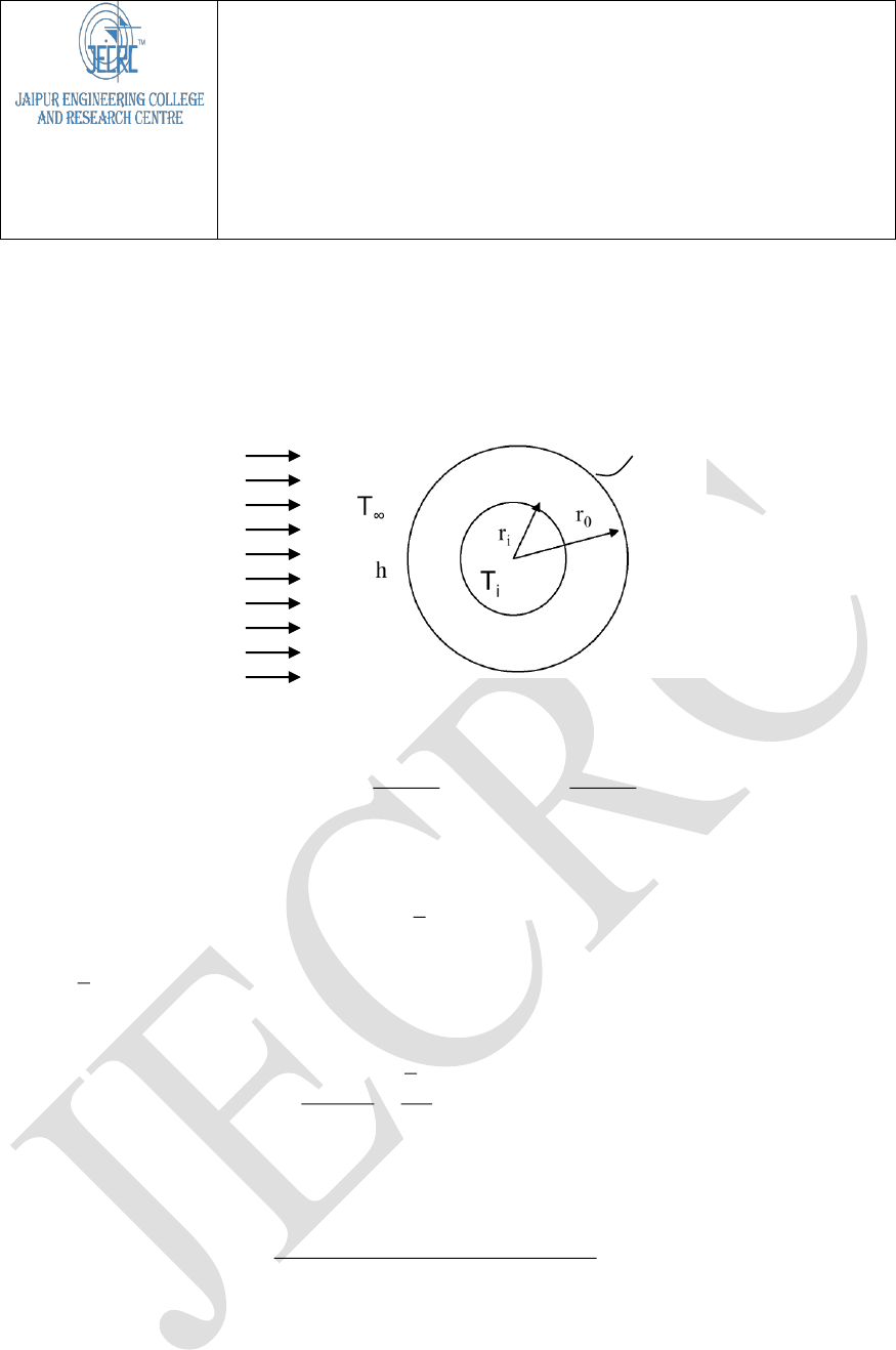
JAIPUR ENGINEERING COLLEGE AND RESEARCH CENTRE
JECRC Campus, Shri Ram Ki Nangal, Via-Vatika, Jaipur
Lumped Heat Capacity
For very large r
i
, the heat transfer rate by conduction through the cylinder wall is
approximately
−
=
−
−
−
L
TT
lrk
rr
TT
lrkq
si
o
io
is
o
)2()2(
(5.3)
where l is the length of the cylinder and L is the material thickness. The rate of heat transfer
away from the outer surface by convection is
))(2(
−= TTlrhq
so
(5.4)
where
h
is the average heat transfer coefficient for convection from the entire surface.
Equating (5.3) and (5.4) gives
k
Lh
TT
TT
s
si
=
−
−
= Biot number (5.5)
The Biot number is dimensionless, and it can be thought of as the ratio
flow heat external to resistance
flow heat internal to resistance
Bi =
Whenever the Biot number is small, the internal temperature gradients are also small and a
transient problem can be treated by the “lumped thermal capacity” approach. The lumped
capacity assumption implies that the object for analysis is considered to have a single mass-
averaged temperature.
Fig. 5.1
TT
s

JAIPUR ENGINEERING COLLEGE AND RESEARCH CENTRE
JECRC Campus, Shri Ram Ki Nangal, Via-Vatika, Jaipur
Lumped Heat Capacity
In the derivation shown above, the significant object dimension was the conduction path
length,
io
rrL −=
. In general, a characteristic length scale may be obtained by dividing the
volume of the solid by its surface area:
s
A
V
L =
(5.6)
Using this method to determine the characteristic length scale, the corresponding Biot
number may be evaluated for objects of any shape, for example a plate, a cylinder, or a
sphere. As a thumb rule, if the Biot number turns out to be less than 0.1, lumped capacity
assumption is applied.
In this context, a dimensionless time, known as the Fourier number, can be obtained by
multiplying the dimensional time by the thermal diffusivity and dividing by the square of the
characteristic length:
Fo
t
time essdimensionl ==
2
L
(5.7)
Lumped thermal capacity analysis
The simplest situation in an unsteady heat transfer process is to use the lumped capacity
assumption, wherein we neglect the temperature distribution inside the solid and only deal
with the heat transfer between the solid and the ambient fluids. In other words, we are
assuming that the temperature inside the solid is constant and is equal to the surface
temperature.
Solid
T(t)
, c, V
Fig. 5.2
T
)(
−= TTAhq
s
h

JAIPUR ENGINEERING COLLEGE AND RESEARCH CENTRE
JECRC Campus, Shri Ram Ki Nangal, Via-Vatika, Jaipur
Lumped Heat Capacity
The solid object shown in figure 5.2 is a metal piece which is being cooled in air after hot
forming. Thermal energy is leaving the object from all elements of the surface, and this is
shown for simplicity by a single arrow. The first law of thermodynamics applied to this
problem is
=
dtdt timeduringobject ofenergy
thermalinternal of decrease
timeduring
object ofout heat
Now, if Biot number is small and temperature of the object can be considered to be uniform,
this equation can be written as
cVdTdtTtTAh
s
−=−
)(
(5.8)
or,
( )
dt
cV
Ah
TT
dT
s
−=
−
(5.9)
Integrating and applying the initial condition
i
TT =)0(
,
t
cV
Ah
TT
TtT
s
i
−=
−
−
)(
ln
(5.10)
Taking the exponents of both sides and rearranging,
bt
i
e
TT
TtT
−
=
−
−)(
(5.11)
where
cV
Ah
b
s
=
(1/s) (5.12)
Rate of convection heat transfer at any given time t:
−= TtThAtQ
s
)()(
Total amount of heat transfer between the body and the surrounding from t=0 to t:
i
TtTmcQ −= )(
Maximum heat transfer (limit reached when body temperature equals that of the
surrounding):
i
TTmcQ −=
5.4 Numerical methods in transient heat transfer: The Finite Volume Method

JAIPUR ENGINEERING COLLEGE AND RESEARCH CENTRE
JECRC Campus, Shri Ram Ki Nangal, Via-Vatika, Jaipur
Lumped Heat Capacity
Consider, now, unsteady state diffusion in the context of heat transfer, in which the
temperature, T, is the scalar. The corresponding partial differential equation is:
S
x
T
k
xt
T
c +
=
(5.13)
The term on the left hand side of eq. (5.13) is the storage term, arising out of
accumulation/depletion of heat in the domain under consideration. Note that eq. (5.13) is a
partial differential equation as a result of an extra independent variable, time (t). The
corresponding grid system is shown in fig. 5.3.
Fig. 5.3: Grid system of an unsteady one-dimensional computational domain
In order to obtain a discretized equation at the nodal point P of the control volume,
integration of the governing eq. (5.13) is required to be performed with respect to time as
well as space. Integration over the control volume and over a time interval gives
+++
+
=
tt
t CV
tt
t cv
tt
t CV
dtSdVdtdV
x
T
k
x
dtdV
t
T
c
(5.14)
P
W
E
x
w
e
(x)
w
(x)
e
t
x

JAIPUR ENGINEERING COLLEGE AND RESEARCH CENTRE
JECRC Campus, Shri Ram Ki Nangal, Via-Vatika, Jaipur
Lumped Heat Capacity
Rewritten,
( )
+++
+
−
=
tt
t
tt
t
we
e
w
tt
t
dtVSdt
x
T
kA
x
T
kAdVdt
t
T
c
(5.15)
If the temperature at a node is assumed to prevail over the whole control volume, applying
the central differencing scheme, one obtains:
( )
( )
++
+
−
−
−
=−
tt
t
tt
t
w
WP
w
e
PE
e
old
P
P
new
dtVSdt
x
TT
Ak
x
TT
AkVTTc
(5.16)
Now, an assumption is made about the variation of T
P
, T
E
and T
w
with time. By generalizing
the approach by means of a weighting parameter f between 0 and 1:
( )
tfftdt
tt
t
old
P
new
PPP
−−==
+
1
(5.17)
Repeating the same operation for points E and W,
xS
x
TT
k
x
TT
kf
x
TT
k
x
TT
kfx
t
TT
c
w
old
W
old
P
w
e
old
P
old
E
e
w
new
W
new
P
w
e
new
P
new
E
e
old
P
new
P
+
−
−
−
−+
−
−
−
=
−
)1(
(5.18)
Upon re-arranging, dropping the superscript “new”, and casting the equation into the standard
form:
bTafafaTffTaTffTaTa
old
PEWP
old
EEE
old
WWWPP
+−−−−+−++−+= )1()1()1()1(
0
(5.19)
where

JAIPUR ENGINEERING COLLEGE AND RESEARCH CENTRE
JECRC Campus, Shri Ram Ki Nangal, Via-Vatika, Jaipur
Lumped Heat Capacity
( )
0
PEWP
aaaa ++=
;
t
x
ca
P
=
0
;
w
w
W
x
k
a
=
;
e
e
E
x
k
a
=
;
xSb =
(5.20)
The time integration scheme would depend on the choice of the parameter f. When f = 0, the
resulting scheme is “explicit”; when 0 < f ≤ 1, the resulting scheme is “implicit”; when f = 1,
the resulting scheme is “fully implicit”, when f = 1/2, the resulting scheme is “Crank-
Nicolson” (Crank and Nicolson, 1947). The variation of T within the time interval ∆t for the
different schemes is shown in fig. 5.4.
Fig. 5.4: Variation of T within the time interval ∆t for different schemes
Explicit scheme
Linearizing the source term as
old
ppu
TSSb +=
and setting f = 0 in eq. (5.19), the explicit
discretisation becomes:
u
old
PEWP
old
EE
old
WWPP
STaaaTaTaTa ++−++= )(
0
(5.21)
where
t
T
T
P
old
t
T
P
new
t+t
f=0
f=1
f=0.5

JAIPUR ENGINEERING COLLEGE AND RESEARCH CENTRE
JECRC Campus, Shri Ram Ki Nangal, Via-Vatika, Jaipur
Lumped Heat Capacity
0
PP
aa =
;
t
x
ca
P
=
0
;
w
w
W
x
k
a
=
;
e
e
E
x
k
a
=
(5.22)
The above scheme is based on backward differencing and its Taylor series truncation error
accuracy is first-order with respect to time. For stability, all coefficients must be positive in
the discretized equation. Hence,
0)(
0
−+−
PEWP
Saaa
or,
0)( +−
e
e
w
w
x
k
x
k
t
x
c
or.
x
k
t
x
c
2
or,
k
x
ct
2
)(
2
(5.23)
The above limitation on time step suggests that the explicit scheme becomes very expensive
to improve spatial accuracy. Hence, this method is generally not recommended for general
transient problems. Nevertheless, provided that the time step size is chosen with care, the
explicit scheme described above is efficient for simple conduction calculations.
Crank-Nicolson scheme
Setting f = 0.5 in eq. (5.19), the Crank-Nicolson discretisation becomes:
bT
a
a
a
TT
a
TT
aTa
P
W
E
P
old
WW
W
old
EE
EPP
+
−−+
+
+
+
=
00
2222
(5.24)
where

JAIPUR ENGINEERING COLLEGE AND RESEARCH CENTRE
JECRC Campus, Shri Ram Ki Nangal, Via-Vatika, Jaipur
Lumped Heat Capacity
PPWEP
Saaaa
2
1
)(
2
1
0
−++=
;
t
x
ca
P
=
0
;
w
w
W
x
k
a
=
;
e
e
E
x
k
a
=
;
old
ppu
TSSb
2
1
+=
(5.25)
The above method is implicit and simultaneous equations for all node points need to be
solved at each time step. For stability, all coefficient must be positive in the discretized
equation, requiring
2
0
WE
P
aa
a
+
or,
k
x
ct
2
)(
(5.26)
The Crank-Nicolson scheme only slightly less restrictive than the explicit method. It is based
on central differencing and hence it is second-order accurate in time.
The fully implicit scheme
Setting f = 1 in eq. (5.19), the fully implicit discretisation becomes:
old
PPWWEEPP
TaTaTaTa
0
++=
(5.27)
where
PWEPP
Saaaa −++=
0
;
t
x
ca
P
=
0
;
w
w
W
x
k
a
=
;
e
e
E
x
k
a
=
(5.28)
A system of algebraic equations must be solved at each time level. The accuracy of the
scheme is first-order in time. The time marching procedure starts with a given initial field of
the scalar
0
. The system is solved after selecting time step Δt. For the implicit scheme, all
coefficients are positive, which makes it unconditionally stable for any size of time step.
Hence, the implicit method is recommended for general purpose transient calculations
because of its robustness and unconditional stability.
APPLICATION:

JAIPUR ENGINEERING COLLEGE AND RESEARCH CENTRE
JECRC Campus, Shri Ram Ki Nangal, Via-Vatika, Jaipur
Lumped Heat Capacity
The application of a simple lumped model to unsteady cooling (or heating) processes in
solids involving heat convection is limited by the value of the Biot number, Bi. ... The Biot
limits depend on the thermal process (heating or cooling) and on the type of temperature
dependence—positive or negative.
EXPECTED OUTCOME:
We have studied the importance and validity of engineering assumptions through the
lamped heat capacity method.
COMMENT BY STUDENT:
VIVA VOCE:
1. What is Lumped heat capacity?
2. What is finite volume method?
3. What is Biot Number?
4. Explain fourier number?
5. What is the thermal diffusivity?
