Pockets of risk in European housing markets: then and now

Working Paper Series

No 87 / February 2019

Pockets of risk in

European housing markets:

then and now

Jane Kelly

Julia Le Blanc

Reamonn Lydon

Abstract

Using household survey data, we document evidence of a loosening of credit

standards in Euro area countries that experienced a property price boom-and-bust

cycle. Borrowers in these countries exhibited signiﬁcantly higher loan-to-value (LTV)

and loan-to-income (LTI) ratios in the run up to the ﬁnancial crisis, and an increasing

tendency towards longer-term loans compared to borrowers in other countries. In

recent years, despite the long period of historically low interest rates and substantial

house price increases in some countries, we do not ﬁnd similar credit easing as

before the crisis. Instead, we ﬁnd evidence of a considerable change in borrower

characteristics since 2010: new borrowers are older and have higher incomes than

before the crisis.

JEL classiﬁcation: E5, G01, G17, G28, R39. Keywords: real estate markets,

macroprudential policy, systemic risk, ﬁnancial crises, bubbles, ﬁnancial regulation,

ﬁnancial stability indicators.

Nontechnical Summary

The ﬁnancial crisis has sparked interest of policymakers and academics alike in analysing

the liability side of households’ balance sheets in order to understand why households

in some countries were hit by the boom-bust episode of the ﬁnancial crisis while others

were not. While comparable household-level data do not exist for the crisis years, we

extract historical information at the country level on lending standards and borrower

characteristics from the Household Finance and Consumption Survey (HFCS). These

micro data can be used to analyse distributions and thus the build-up of potential tail

risks. The goal of this paper is to explore how such household-level micro data can be

used for understanding macro-ﬁnancial risks and linkages and eventually to mitigate

risks through macroprudential policies in place.

We document the heterogeneous experiences of households in the Euro area in the run

up to the ﬁnancial crisis and after the bust. Following the literature, we divide countries

into two groups: those that experienced a house price boom (Greece, Spain, Ireland, Italy,

Netherlands, Slovenia, Latvia and Estonia) and those that did not (Belgium, Germany,

France, Luxembourg, Austria and Portugal).

The paper ﬁrst provides evidence of a loosening of credit standards in countries that

experienced a property price boom-and-bust. At the onset of the ﬁnancial crisis,

borrowers in these countries exhibited signiﬁcantly higher loan-to-value (LTV) and loan-

to-income (LTI) ratios: 40-50% of all household main residence mortgages had LTVs of

90% or more, and both LTI ratios and loan terms had increased. Credit easing persisted

when house prices increased and consequently induced high indebtedness and more

credit expansion, which resulted in substantial pockets of risk before the Great Financial

Crisis hit. In contrast, households in countries without a boom in real estate prices

experienced no comparable declines in credit standards and most did not see substantial

house price increases before and during the crisis.

Second, the paper analyses the composition of buyers in both country groups before and

after the crisis. The loosening of credit standards before 2010 shifted the composition of

buyers in boom-bust countries towards younger households with relatively low incomes

compared to the group of countries without a housing boom. Contrary to this, we

ﬁnd evidence of a considerable change in borrower characteristics since 2010: new

borrowers have become older and have higher incomes than before the crisis in most

countries.

The paper then describes the impact of indebtedness on credit constraints. We ﬁnd that

borrowers with high levels of leverage are more likely to become credit constrained, and

this effect is stronger for boom-bust countries than for countries that did not experience

a boom before the crisis. In recent years, borrowers with high levels of leverage are more

likely to become credit constrained in both groups.

Finally, the long period of historically low interest rates since the ﬁnancial crisis raises the

question of whether similar pockets of risk have emerged, considering substantial house

price increases in recent years in some countries in our sample. However, we do not

ﬁnd similar credit easing as before the crisis in either group of countries. Instead, there

is some evidence that more afﬂuent households have shifted their portfolios towards

housing at a time when real returns on deposits or other forms of (less) risky investments

are at an all-time low.

1 Introduction

Up until the ﬁnancial crisis, safeguards in Euro area macroeconomic policy primarily

targeted low and stable inﬂation, the prevention of excessive government deﬁcits, and

structural reforms to underpin productivity growth. Potential instabilities arising from

excessive household indebtedness, and ﬁnancial fragility more generally, received far

less attention. The ﬁnancial crisis reinvigorated research into the causes and effects of

ﬁnancial instability, particularly credit-driven real estate boom-bust cycles.

Within the

EMU, the inability of some Member States to credibly back-stop an over-sized domestic

banking system contributed directly to a whole host of negative economic consequences

that continue to be felt today. Policy reforms introduced since the crisis, such as the

Single Supervisory Mechanism (SSM), the European System of Financial Supervision

(ESFS), the EU Bank Recovery and Resolution Directive (BRRD) and ﬁscal governance

reforms (for example, the six-pack, two-pack and ﬁscal compact) have sought to

address some of these weaknesses in the EMU policy infrastructure.

Furthermore,

macroprudential measures at both the Euro area and national levels, which explicitly

recognise risks at the ﬁnancial system level and how such ﬁnancial sector developments

affect the real economy, are becoming increasingly common in Europe.

This includes

measures related to real estate lending which generally aim to build resilience among

households and banks to withstand a shock and to restrain the build-up of excessive

imbalances between credit and real estate markets.

One of the legacies of the inattention to the build-up of household ﬁnancial fragilities

in the early years of EMU is a distinct lack of comparable cross-country data on

borrower and mortgage characteristics. One of the key contributions of this paper is

to ﬁll this information gap. We collate information on credit standards and borrower

characteristics from the ﬁrst two waves of the European Household Finance and

For an overview, see Claessens et al. (2009) or Crowe et al. (2013).

The ESFS comprises the European Systemic Risk Board (ESRB), the European Banking

Authority (EBA), the European Securities and Markets Authority (ESMA) and the European

Insurance and Occupational Pensions Authority (EIOPA). The latter three are jointly referred to

as the European Supervisory Authorities (ESAs).

The ESRB has oversight across the EU. The ECB has topping up powers for certain

macroprudential instruments (such as capital based tools) for banks in SSM countries but

borrower based tools such as loan-to-value (LTV) or debt-to-income (DTI) limits are under the

discretion of national macroprudential authorities.

Limits on loan-to-value (LTV) and debt-to-income (DTI) ratios are found to be particularly

effective in recent cross country empirical studies such as Claessens (2015).

Consumption Survey (HFCS 2010 and 2013), comparing patterns across countries and

time.

Following Hartmann (2015) and the ESRB (2015), countries are separated into

those that experienced a Residential Real Estate (RRE) boom-and-bust (Greece, Spain,

Ireland, Italy, Netherlands, Slovenia, Latvia and Estonia) and those that did not (Belgium,

Germany, France, Luxembourg, Austria and Portugal). Boom-bust countries experienced

an average peak-to-trough fall in house prices of 36%; the peak-to-trough fall in non

boom-bust countries was just 4% (see Table 1 for country-speciﬁc data). ESRB (2015)

point out that most of the boom-bust countries also experienced a real estate related

banking crisis following the Global Financial Crisis (GFC) with severe consequences for

the real economy (the one exception is Estonia).

TABLE 1. Peak-to-trough house price changes

Peak year Peak (2010=100) Trough ∆Peak-trough Boom-bust

Ireland 2007 143.2 70.4 -50.8% Yes

Estonia 2007 187.1 98.3 -47.4% Yes

Greece 2007 117.5 67.1 -42.9% Yes

Spain 2007 115.7 67.5 -41.7% Yes

Netherlands 2008 116.5 81.1 -30.4% Yes

Slovenia 2008 112.9 81.4 -27.9% Yes

Italy 2007 107.5 80.2 -25.4% Yes

Lativa 2007 121.3 100.0 -17.6% Yes

Portugal 2007 105.0 90.4 -13.9% No

France 2011 104.1 95.7 -8.1% No

Belgium 2013 101.5 100.2 -1.3% No

Germany 2015 123.7 123.7 0.0% No

Luxembourg 2015 124.8 124.8 0.0% No

Austria 2015 100.0 100.0 0.0% No

Boom-bust -35.5%

Non-boom-bust -3.9%

Excl. Portugal -1.6%

Source: OECD data on real house prices.

Notes: The HFCS contains data for 15 countries in Wave 1 (2010) and 20 countries in Wave 2 (2014). We exclude the

following countries: Poland, Hungary and Slovak Republic (outside the Euro Area for some/all of the sample period);

Malta (small cell sizes for historic purchases); Cyprus (small sizes after 2010).

Our paper sheds new light on the sources of real estate boom-bust cycles in several

different dimensions. We compare measures such as mean loan-to-value (LTV) and loan-

In a prescient paper, Fagan and Gaspar (2005) show that many of the RRE boom-bust

countries also experienced a large reduction in nominal interest rates upon joining the single

currency. They highlighted the potential ﬁnancial instability risks arising from a rapid drop in

borrowing costs as a potentially negative side-effect of increased ﬁnancial integration.

to-income (LTI) ratios, and we look at distributions and thus at the build-up of potential

tail risks. Understanding the evolution of these tail risks is important because countries

that have introduced borrower-based macro-prudential measures in recent years – such

as LTV or LTI caps – target these tail risks. Looking at the entire distribution of borrowers

provides important additional insights over averages and addresses questions such as

whether particular borrower cohorts are more vulnerable (e.g. younger or low income

groups) and of whether signs of credit easing can be observed along multiple dimensions

(e.g. longer loan terms alongside higher LTVs).

As well as ﬁlling key data gaps, our paper contributes to two other literatures on

how credit standards affect households and the economy more widely. First, we show

that more indebted borrowers are signiﬁcantly more likely to face credit constraints

following an income shock with negative consequences for household spending, similar

to the results in Dynan (2012) and Mian and Suﬁ (2015). Second, we provide cross-

country evidence on how borrower composition both affects, and is affected by credit

standards, building on papers by Laeven and Popov (2017) and Lydon and McCann

(2017).

Our results are informative for early warning models of future vulnerabilities. ESRB

(2015), Behn et al. (2016), Claessens (2015) and Cerutti et al. (2015) all highlight the

usefulness of micro-based measures of indebtedness such as loan-to-value (LTV) and

loan-to-income (LTI) ratios both as early warning indicators and as macro-prudential

policy tools.

However, the formal adoption of ‘borrower-based’ macroprudential

policies is relatively recent in many Euro area countries and empirical evidence remains

scarce.

Most studies focus on whether a policy was in place or not, rather than the

intensity of the policy relative to the prevailing regime beforehand. Our time-series

evidence could help calibrate future policies. A cross-country perspective may also be

helpful for informing public debate when measures are enacted, as the short-term costs

At the country level, the Central Bank of Ireland has combined administrative data on loans

with historical survey data – including the HFCS – to understand exactly how macro-ﬁnancial

linkages operate. See, amongst others, Le Blanc (2016), Kelly and Lydon (2017), Byrne et al.

(2017), Kelly et al. (2015), Coates et al. (2015), Cussen et al. (2015) and CBI (2016). Similar

country-level studies in other EA countries include Albacete et al. (2014) (Austria), Costa and

Farinha (2012) (Portugal), de Caju (2016) (Belgium) and Room and Merikall (2017) (Estonia).

Note, borrower-based macroprudential rules are distinct from rules or non-binding

recommendations associated with particular types of mortgage lending. The latter would include

LTV limits traditionally applicable to lending used as collateral for covered bonds, limits in place

for lending granted by certain types of lenders such as Building Societies or for mortgages insured

by the government, or supervisory recommended best practice guidelines rather than strictly-

enforced rules.

– such as the additional time required to save for a deposit – are often more visible than

the long-term beneﬁts (higher household resilience to house price or income shocks).

Our ﬁndings can be summarised as follows: For countries that experienced a real

estate boom-and-bust (Estonia, Ireland, Greece, Spain, Cyprus, Italy, Latvia, Netherlands

and Slovenia), there is clear evidence of a deterioration of credit standards before the

Financial Crisis: around half of all household main residence (HMR) mortgages had LTVs

of 90% or more, and both LTI ratios and loan terms increased. Borrowers with high

origin LTVs also exhibit higher debt service burdens, particularly among lower income

(often younger) households. After 2008, and despite the prevailing low interest rate

environment, we observe a sharp tightening of lending standards in the boom-bust

countries with a decline in LTVs, LTIs and loan terms. In many countries, this pre-dates

the introduction of explicit borrower based macroprudential limits. In contrast, we

ﬁnd broadly constant credit standards across the entire period we analyse (2000-2014)

in non-boom-bust countries (Belgium, Germany, France, Luxembourg, Malta, Austria,

Portugal and Slovakia). In addition to the systemic risks arising from a loosening of

credit standards, we show that following an income shock, more indebted households

are signiﬁcantly more likely to be credit constrained. This is clear evidence of one of the

channels through which over-indebtedness can weigh on economic activity.

Shifting attention to the more recent period of very low interest rates, we observe

no comparable loosening of lending standards. Instead, we observe a shift in borrower

composition towards older and higher income borrowers, irrespective of the country

that households live in. In the majority of countries, the top two income quintiles account

for roughly 70 per cent of mortgages in the more recent period, and the percentage

of borrowers aged over 40 has increased. The reasons for such a shift in borrower

composition vary. In boom-bust countries, the shift appears to be due to a tightening of

credit standards after the bust, which has made it more difﬁcult for younger and lower-

income borrowers to obtain a mortgage. In non-boom-bust countries the dramatic fall in

the cost of capital for housing due to the low interest rate environment may have shifted

household portfolios from relatively low-return ﬁnancial assets into higher-return real

assets.

The remainder of the paper is structured as follows. Section 2 gives an overview

of the HFCS dataset and explains how we construct the key variables in our analysis.

Section 3 uses this data to revisit the evolution of credit standards during the boom-bust

cycles and more recently. Section 4 focuses on shifts in borrower composition. Section

5 examines the relationship between borrower leverage and credit constraints from a

cross-country perspective. Finally, Section 6 concludes.

2 Data – the Household Finance and Consumption Survey

The Household Finance and Consumption Survey (HFCS) is primarily a wealth survey with

detailed information on income, assets, debts and the repayment burden on debt. The

ﬁeldwork for the ﬁrst wave, covering 15 countries, took place in 2010 for most countries;

the second wave, which expanded the survey to a further ﬁve countries, took place in

2014 for most countries. Table 2 provides an overview of the data; two ECB reports,

ECB (2013) and ECB (2016), summarise the results from each wave.

TABLE 2. The Household Finance and Consumption Survey (HFCS)

Survey # households # households with % households with

years pooled any mortgage debt mortgage debt

Belgium 2010, 2014 4,565 1,329 33%

Germany 2010, 2014 8,026 2,292 21%

Estonia 2013 2,220 566 21%

Ireland 2013 5,419 2,056 37%

Greece 2009, 2014 5,974 861 15%

Spain 2008, 2012 12,303 3,284 34%

France 2010, 2014 27,041 7,650 24%

Italy 2010, 2014 16,107 1,409 10%

Latvia 2014 1,202 250 17%

Luxembourg 2010, 2014 2,551 1,069 37%

Netherlands 2009, 2014 2,585 1,386 43%

Austria 2010, 2014 5,377 840 18%

Portugal 2010, 2013 10,611 3,484 36%

Slovenia 2014 2,895 285 11%

Source: HFCS waves 1 and 2. For countries with two waves of data, the ﬁgures relate to the pooled datasets.

The degree of access to detailed micro-level data varies considerably across the EU

and national macroprudential authorities.

In some Member States, detailed micro-

data is available from the loan books of domestic banks or from central credit registers.

For other countries, evidence has often relied upon bank surveys (for example Austria,

Belgium, Finland and France). One of the difﬁculties for cross-country studies is that the

For example, the Deutsche Bundesbank noted in its 2016 Financial Stability Review that

access to granular data is limited and that the responsible authorities in Germany lacked the

means to set minimum standards for the issuance of housing loans as a targeted macroprudential

policy measure. See “Box on Macroprudential Policy Making Procedure”.

deﬁnition of variables often differs not only between banks but also across countries.

The ESRB (2015) has compiled average statistics on LTV ratios for selected EU countries

but warns that such estimates are based on divergent concepts.

Differences may arise

across lending types (e.g. new vs. outstanding lending and in some cases including credit

lines), borrower types (First-time borrowers (FTBs) vs. all borrowers, Owner Occupiers

or include Buy-to-Lets (BTLs)), loan purpose (purchasing, renovating), aggregation level

(a loan, collateral or borrower view) and valuation concepts (origin, current and indexed

LTV). Similarly for income based measures, such as debt service to income (DSTI) and

loan or debt to income ratios (LTI or DTI) income can be deﬁned on a gross or a net basis

and include or exclude living expenses, bonuses and rental income.

We use the HFCS to extract historical information at the country level on lending

standards and borrower characteristics. In this respect, the HFCS has some clear

advantages over other potential data sources. For example, compared to RMBS pool

data which may account for a smaller share of mortgage lending in some countries, it

should be more representative of borrowers in any given year; see Thebault (2017).

Furthermore, because we are using the same underlying survey data for all countries

cross-country comparability should be less of a concern, in comparison to other studies,

such as ESRB (2016) and ESRB (2015). However, the HFCS is not without potential

problems. In terms of this exercise, we can think of two speciﬁc issues: (i) measurement

error arising from recall problems; and (ii) survival bias. We discuss each in turn.

Recall issues

We use survey responses on property purchase price and loan drawn down at

origination to construct historical LTV ratios. Accurately recalling historical ﬁnancial

information can be difﬁcult for some households, potentially leading to non-response

and measurement error. Item non-response to these questions is relatively low in most

countries, at less than 5% of households in the dataset. For a non-response item in the

HFCS, multiple imputation (MI) is used. We have run the analysis in this paper with

and without the imputed observations, and our results do not change. Measurement

error could be problematic if it is correlated with events such as house price booms-and-

busts. However, comparing the historical house prices series with other sources such

as the OECD (see Figure 1) suggests HFCS trends closely track other published data.

See, for example, ESRB Report on residential real estate and ﬁnancial stability in

the EU (2015), ESRB Handbook on operationalising macro-prudential policy (2014), ESRB

Vulnerabilities in the EU residential real estate sector (2016).

The ﬁrst chart in Figure 1 compares house price trends in the HFCS for all countries

with those from the OECD; the second chart is for non boom-bust countries and the

ﬁnal chart is for boom-bust countries.

As well as the original house price, we also use

information on the original loan drawn-down to construct the Loan-to-Value ratio (LTV)

at origination. As discussed earlier, there is limited external information against which

we can validate the HFCS trends on mortgage size at origination. However, country-

speciﬁc assessments of the information on debt in the HFCS show that it is comparable

with data from administrative sources; see Kelly and Lydon (2017) for Ireland and

Albacete et al. (2016) for Austria.

Survival bias

The HFCS dataset is a snapshot of households’ balance sheets and incomes in 2010

(wave 1) and 2014 (wave 2). We rely on households who have mortgage debt in each

wave to construct historic trends in lending standards. Survival bias can arise if loans

originating in a given year do not appear in either snapshot – in other words, if some

loans are repaid (or defaulted) between the origination year and the survey year.

For LTVs, this could bias past values upwards if loan term and originating LTV are

positively correlated, as they tend to be. However, the comparable data that is available

for individual countries does not lead us to believe that the potential biases are large.

For example, in the case of Ireland, Kelly and Lydon (2017) show that historical LTVs

extracted from the HFCS track loan-level administrative data very closely. Albacete et al.

(2014) carries out a similar comparison for Austrian households and ﬁnds that the HFCS

data tracks administrative data on average loan size (and LTV) quite closely. Beyond

these publications, there is little published information against which we can compare

the historical HFCS information – indeed, this is one of the motivations for the current

exercise. We have done a comparison of the volume of new business loans for house

purchase from the ECB Statistical Data Warehouse (SDW) with the HFCS. Whilst the

trends are very similar across countries and time, the levels are quite different due to

the fact that the deﬁnition of ‘new business’ in the SDW is not really comparable to new

loans drawn down in the HFCS, as it includes interest rate resets, renegotiations and not-

for proﬁts serving households.

Figure 17 in the appendix compares house price trends for each individual country in our

sample with external sources. In all cases, we ﬁnd that HFCS trends very closely track other data

sources.

FIGURE 1. House price trends (2008=100)

100

Nominal house price index (2008=100)

1995 2000 2005 2010 2015

HFCS data

OECD data

House price trends in OECD and HFCS data

100

120

Nominal house price index (2008=100)

1995 2000 2005 2010 2015

HFCS data

OECD data

House prices: HFCS-v-OECD, non RRE boom-bust countries

100

120

Nominal house price index (2008=100)

1995 2000 2005 2010 2015

HFCS data

OECD data

House prices: HFCS-v-OECD, RRE boom-bust countries

Source: HFCS, waves 1 and 2 and OECD. The nominal price indices are means of HMR

property purchase price by year of purchase for all mortgage-ﬁnanced purchases.

The following countries are in the boom-bust group: Estonia (from 2004 in HFCS

data), Ireland, Greece, Spain, Cyprus, Italy, Latvia (from 2004), Netherlands and

Slovenia (from 2004). The non-boom-bust group of countries are: Belgium, Germany,

France, Luxembourg, Malta, Austria, Portugal and Slovakia.

3 Credit Standards for Residential Real Estate (RRE)

This section highlights that property bubbles and changes in credit standards go hand-

in-hand. In the following, we analyse the HFCS to see whether common patterns

emerge among our boom-bust group that might have triggered concerns at that time and

whether we observe any comparable broad-based easing of credit standards in the more

recent period. Figures 2 (boom-bust countries) and 3 (non-boom bust) provide context

for the analysis: using OECD data, we present a top-down picture of trends in real house

prices, house price-to-disposable income ratios and household debt-to-income ratios for

the countries in the sample. A number of patterns emerge:

Ireland, Estonia, Lativa and Spain stand out as countries that experienced large

real-estate boom-and-busts. The run-up in house prices in these countries far

surpassed income growth, and was fuelled to a large degree by rapid growth in

household debt.

Relative to incomes, house prices in non-boom-bust countries also increased

during the early-2000s, albeit at about half the rate seen in boom-bust countries.

Since 2010, Germany, Austria, Luxembourg and, to a lesser extent, Belgium are the

only countries (in the non-boom bust group) with signiﬁcant house price increases

both in absolute levels and relative to incomes (middle panel). As the ﬁnal panel

(debt-to-income ratio) shows, however, this recent run-up in house prices does not

appear to have been accompanied by a large increase in debt, with debt-to-income

ratios either increasing more slowly or not at all.

LTV at origination

Figure 4 shows the rise in the share of new ‘Household Main Residence’ (HMR)

mortgages with an LTV of 90 per cent or higher in the boom-bust group in the run-up

to the GFC: at the peak, such mortgages account for just over 50 per cent of new lending.

In contrast, the trend for the non-boom-bust country group is relatively stable over time,

at between 30 and 35 per cent of loans. Figure 5 shows the same data for the pre- (2006-

08) and post- (2011 onwards) crisis period for individual countries.

Portugal experienced an earlier credit boom (1995-2005), also covering consumer credit,

not just mortgage credit. See Blanchard (2007) and Reis (2013) for more in-depth discussion on

the Portuguese experience.

FIGURE 2. House prices, house-price-to-income ratio and debt-to-income ratio:

countries that experienced a property boom-and-bust

100

150

200

Real house prices

1995 2000 2005 2010 2015

Ireland

Greece

Spain

Italy

Netherlands

Latvia

Estonia

Slovenia

100

150

200

House price-to-income

1995 2000 2005 2010 2015

Ireland

Greece

Spain

Italy

Netherlands

Latvia

Estonia

Slovenia

100

200

300

Debt-to-income ratio

1995 2000 2005 2010 2015

Ireland

Greece

Spain

Italy

Netherlands

Latvia

Estonia

Slovenia

Source: OECD housing and income statistics and authors’ calculations. The house-price to income ratio is

relative to its long-run mean, with 2010=100.

FIGURE 3. House prices, house-price-to-income ratio and debt-to-income ratio:

countries that did not experience a property boom-and-bust

100

120

140

Real house prices

1995 2000 2005 2010 2015

Belgium

Germany

France

Luxembourg

Austria

Portugal

Finland

100

120

140

House price-to-incomes ratio

1995 2000 2005 2010 2015

Belgium

Germany

France

Luxembourg

Austria

Portugal

Finland

100

120

140

Debt-to-income ratio

1995 2000 2005 2010 2015

Belgium

Germany

France

Luxembourg

Austria

Portugal

Finland

Source: OECD housing and income statistics and authors’ calculations. The house-price to income ratio is

relative to its long-run mean, with 2010=100.

Countries that experienced a housing boom-bust saw a contraction in the share of

very high LTV loans after the housing bubble burst. In countries like Ireland, for example,

the proportion of these 90%-plus loans fell by more than a half, from just under 50% of

loans to less than 20%. The share of high-LTV loans is more stable over time in non boom-

bust countries, with the exception of Portugal. Real house prices in Portugal did fall

during the ﬁnancial crisis, but this appears to be part of a longer-term trend, beginning in

the early 2000s.

FIGURE 4. Percentage of HMR loans with an LTV of 90% plus

% HMR loans>90 LTV

1995 2000 2005 2010 2015

Boom-bust countries

Non Boom-bust countries

Source: HFCS, waves 1 and 2. New loans for house purchase, i.e. excludes reﬁnancing, renegotiating or

topping-up existing loans.

FIGURE 5. Percentage of HMR loans with an LTV of 90% plus at origination (by country)

10%

20%

30%

40%

50%

60%

AT DE FR BE LU PT SI IT ES LV GR EE IE NL

Percentage of loans with an LTV>90% at

origination

2004-08 2011 onwards

No RRE boom-bust

RRE boom-bust

Source: HFCS, waves 1 and 2.

One challenge that arises when comparing loan characteristics across time is to identify

separately changes in credit standards from changes in borrower composition. Using

the HFCS, we observe substantial shifts in borrower composition in many countries –

and not just those countries that experienced a property boom-bust – with a general

shift towards older and higher-income buyers (see section 4, which discusses the

compositional shifts in more detail).

To get a sense of the importance of compositional factors for these changes, we

plot the percentage of high-LTV loans (≥ 90% LTV) by income quintile and age for

loans originating between 2004 and 2008 (when we expect credit standards were

looser in boom-bust countries) and loans originating from 2011-14 (when we expect

to see a tightening of standards). Compared to non boom-bust countries, there is

a clear reduction in average LTVs at origination in boom-bust countries after 2011.

Importantly, from the perspective of compositional shifts, this pattern of changes is

broadly consistent across the income and age distribution, indicating that the change in

buyer characteristics is not the primary reason we observe a general tightening of credit

standards in the bust.

FIGURE 6. Percentage of HMR loans with an LTV of 90% plus at origination (by income

and age)

10%

20%

30%

40%

50%

60%

70%

1 2 3 4 5

Percentage of loans with LTV>90 by income quintile

Boom-bust countries

Loans 2004-08 Loans 2011-14

Income quintile

10%

20%

30%

40%

50%

60%

70%

1 2 3 4 5

Percentage of loans with LTV>90 by income quintile

Non boom-bust countries

Loans 2004-08 Loans 2011-14

Income quintile

10%

20%

30%

40%

50%

60%

70%

30 35 40 45 50 55 60

Percentage of loans with LTV>90 by age

Boom-bust countries

Loans 2004-08 Loans 2011-14

Age

10%

20%

30%

40%

50%

60%

70%

30 35 40 45 50 55 60

Percentage of loans with LTV>90 by age

Non boom-bust countries

Loans 2004-08 Loans 2011-14

Age

Source: HFCS. Dashed lines show the 95% conﬁdence interval of the mean.

We can also use a regression to control for changes in borrower characteristics, as in

Table 3. The ﬁrst column is an OLS regression of LTV at origination on characteristics

(age, education and income) and a dummy variable interaction for boom-bust countries

and loans drawn-down after 2010. The absolute swing in average LTVs from boom-to-

bust is given by summing the coefﬁcients on the 2004-08 and 2011-14 periods. The

coefﬁcients suggest a fall in average LTVs in boom-bust countries after 2010 of 14

percentage points. The second column is a probit model where the dependent variable

equals one if the loan at origination was 90 per cent or more of the property purchase

price (i.e. LTV≥90). The coefﬁcients conﬁrm the patterns shown in the earlier charts,

that of a sharp contraction in LTVs in boom-bust countries after the crash. The ﬁnal

column is similar to the second, but we restrict the sample to borrowers under the age

of 40. Given that younger borrowers are likely to have a lower level of savings for

a downpayment, we expect a larger coefﬁcient on the dummy variable for the post-

2010 period in boom-bust countries, which is indeed what we ﬁnd. Interestingly, the

regression results also suggest a tightening of LTVs in non boom-bust countries after

2010. This suggests that our observation of relatively unchanged credit standards in

these countries – certainly in the period after 2010 – is partially driven by the greater

concentration of older- and higher-income borrowers, a trend we discuss in more detail

below.

TABLE 3. Average LTV at origination and borrower characteristics

(1) (2) (3)

Dependent variable LTV LTV>=90 LTV>=90

Model OLS Probit* Probit*

All ages All ages Age<40

Non boom-bust countries

Loans originating 2004-08 [Omitted] [Omitted] [Omitted]

Loans originating 2011-14 -4.586*** -0.0533*** -0.0456***

(0.900) (0.0137) (0.0177)

Boom-bust countries

Loans originating 2004-08 10.36*** 0.0463*** 0.0532***

(0.688) (0.0080) (0.00979)

Loans originating 2011-14 -3.702*** -0.0496** -0.0681***

(1.385) (0.0250) (0.0322)

Age -0.297*** -0.00719*** -0.0090***

(0.0315) (0.0003) (0.0006)

Primary education [Omitted] [Omitted] [Omitted]

Secondary education -3.143** -0.0617*** -0.0717***

(1.394) (0.0171) (0.0219)

Post-secondary education -9.353*** -0.131*** -0.144***

(1.212) (0.0149) (0.0191)

Tertiary education -11.10*** -0.147*** -0.155***

(1.251) (0.0156) (0.0198)

Log(income) -2.423*** -0.0501*** -0.0410***

(0.411) (0.00499) (0.0061)

Observations 87,066 78,950 55,560

Standard errors in parentheses. *** p<0.01, ** p<0.05, * p<0.1

Source: HFCS waves 1 and 2. Households with a HMR (‘household main

residence’) mortgage. Loans for house purchase only. (*) The reported

probit results are estimated average marginal effects.

Loan-to Income, Loan terms and debt service ratios

Lenders can change the amount of available credit by lending more (or less) to

households on a given income. This means increasing the loan-to-income ratio (LTI)

and, for a given loan term and interest rate, increasing the debt-service ratio (DSR), the

amount of income devoted to repaying the debt. Whilst the HFCS cross-sections have

information on household income and its components, it is only recorded in the year of

each survey wave. It is therefore not possible to construct a time-series measure of LTI

at origination as we have done for LTV. Instead, we compare the current loan-to-income

ratio for borrowers depending on when the loan originated.

Figure 7 illustrates average LTI by age for loans originating 2004-08 versus 2011-

14. The drop in average LTI after 2010 is evident for the boom-bust group, particularly

for borrowers under 35. For the non-boom bust group, very little change is apparent,

although younger borrowers exhibit higher income multiples than older households.

FIGURE 7. Average HMR Loan-to-income by age

Boom-bust countries

3.00

3.25

3.50

3.75

4.00

4.25

4.50

<35 35-44 45-54 55-64

Loan-to-income ratio by year of loan origination

Boom-bust countries

2004-08

2011-14

Age

Non boom-bust countries

3.00

3.25

3.50

3.75

4.00

4.25

4.50

<35 35-44 45-54 55-64

Loan-to-income ratio by year of loan origination

Non boom-bust countries

2004-08

2011-14

Age

Source: HFCS Waves 1 & 2.

As with LTVs, compositional changes also distort comparisons of LTIs over time. To

control for these changes, we estimate a regression with LTI at origination as the

dependent variable, controlling for age, income and education (Table 4). We include a

dummy variable interaction for boom-bust countries and loans originating after 2010

(when we assume credit standards tightened for boom-bust countries).

TABLE 4. Loan to income ratio and borrower characteristics

(1) (2) (3)

Dependent variable Loan-to-income ratio at survey year

Model OLS OLS OLS

All Age <40 Age ≥ 40

Non Boom-bust countries

Loans originating 2004-08 [Omitted] [Omitted] [Omitted]

Loans originating 2011-14 0.103*** 0.163*** 0.0377

(0.0287) (0.0394) (0.0421)

Boom-bust countries

Loans originating 2004-08 0.115*** -0.00617 0.199***

(0.0210) (0.0310) (0.0289)

Loans originating 2011-14 -0.414*** -0.559*** -0.154**

(0.0470) (0.0600) (0.0755)

Age -0.0259***

(0.000930)

Income Quintile 1 [Omitted] [Omitted] [Omitted]

Income Quintile 2 0.00925 0.168 0.0101

(0.104) (0.198) (0.127)

Income Quintile 3 -0.111 0.173 -0.116

(0.0989) (0.191) (0.118)

Income Quintile 4 -0.379*** -0.242 -0.247**

(0.0976) (0.189) (0.117)

Income Quintile 5 -1.256*** -1.225*** -1.060***

(0.0972) (0.189) (0.116)

Primary education [Omitted] [Omitted] [Omitted]

Secondart education -0.0117 -0.327*** 0.228***

(0.0520) (0.0984) (0.0631)

Post-secondary education -0.266*** -0.367*** -0.0958*

(0.0447) (0.0874) (0.0529)

Tertiary education -0.214*** -0.236*** -0.0890*

(0.0451) (0.0874) (0.0535)

Observations 27,972 12,541 15,431

R-squared 0.130 0.135 0.087

Standard errors in parentheses. *** p<0.01, ** p<0.05, * p<0.1

Source: HFCS waves 1 and 2. Households with a HMR (‘household main

residence’) mortgage. Loans for house purchase only.

The regression results are broadly in line with the trends in the previous two charts.

There is a sharp tightening of loan-to-income ratios in boom-bust countries after the

bursting of the housing bubble in those countries, with a downward swing in LTIs of over

50 basis points. An LTI ratio of about 3.5 – 4.5 can be considered as quite high, although

there is no international benchmark for LTIs and macro-prudential limits on LTI vary

quite considerably in terms of both levels and implementation details.

As the charts

For EU countries that have applied maximum LTI ratios in recent years (Ireland, the UK,

Denmark and the Netherlands) both the limits and the way in which they apply varies. In Ireland,

for example, a maximum of 20 per cent of new residential mortgage lending was allowable at an

LTI of greater than 3.5 times income until end 2017, after which allowances were split among

FTBs and second and subsequent buyers. In the UK, the corresponding ﬁgure is less than 15 per

suggested, the tightening affects mainly younger borrowers, although there is a decline

for older borrowers (≥ 40) bringing them more in-line with average LTIs in non boom-

bust countries. There is also a small increase in average LTIs in non boom-bust countries

after 2010.

One way to ease the debt repayment burden when house prices and indebtedness are

rising faster than income is to extend repayments over a longer period. The increase in

loan terms in some boom-bust countries, such as Ireland, for example, where the average

loan term increased from less than 25 years in the early 2000s to 30 years by 2007, is

suggestive of increasing LTIs over the same period (Figure 8). Looking at the non-boom-

bust group of countries, for example, Austria and Germany, there is very little change in

loan terms over time. In others, such as France, Luxembourg and Belgium, loan terms

increased a little in early- to mid-2000s, before levelling-off.

Households with higher origin LTVs also exhibit signiﬁcantly higher debt-service

burdens; that is, their HMR mortgage repayments represent a high proportion of their

gross income. Figure 9 shows that borrowers on lower incomes tend to have higher debt

service burdens. It also shows the borrowers with the heaviest repayment burden also

have the highest origin LTVs. Low income, high leverage borrowers would appear to be

the most vulnerable to an income or unemployment shock, a result consistent with the

work of Ampudia et al. (2016).

The overall picture is one of a general easing of lending standards in the boom-bust

countries prior to the Great Financial Crisis and a tightening of those standards in the

ensuing years. The regression analysis, which aims to control for compositional changes

in the borrower group suggests a slight loosening of credit standards in non boom-bust

countries after 2010, when we look at Loan-to-income ratios (LTI) – i.e. an increase

in LTIs relative to the mean controlling for characteristics. However, compared with

changes observered in the boom-bust countries in earlier years, these increases are

relatively small. In general, younger and lower income borrowers are the cohorts with

the highest levels of leverage. Next, we consider compositional changes in more detail,

followed by analysis of the consequences for borrowers of taking on too much debt, i.e.

giving rise to credit constraints.

cent at an LTI of greater than 4.5. See ESRB “A review of macroprudential policy in the EU in

2016”, April 2017 for more details on these LTI measures. LTI limits may apply to gross income or

net income and may also differ in what is included in income such as bonuses, rental income and so

forth. One of the beneﬁts of the HFCS is that one can construct reasonably comparable measures

of LTI across countries, notwithstanding the structural differences that exist in mortgage markets

and taxation.

FIGURE 8. Average HMR Loan-terms

Loan term (years)

2000 2005 2010 2015

Estonia

Ireland

Greece

Spain

Italy

Latvia

Netherlands

Slovenia

Loan term (years)

2000 2005 2010 2015

Belgium

Germany

France

Luxembourg

Austria

Portugal

Source: HFCS Wave 1 and 2. Loans for HMR purchase only, i.e. excluding reﬁnancing/renegotiation of existing

loans.

FIGURE 9. HMR mortgage debt-service burden and origin LTV

Boom-bust countries Non-boom-bust countries

Current mortgage debt-service (HMR)

25 50 75 100

LTV at origination

Income Quintile<=2

Quintile=3-4

Quintile=5

Current mortgage debt-service (HMR)

25 50 75 100

LTV at origination

Income Quintile<=2

Quintile=3-4

Quintile=5

Source: HFCS Wave 1 and 2. Debt-service burden as at survey year based on gross income. Loans for HMR

purchase only, i.e. excluding reﬁnancing/renegotiation of existing loans.

4 Borrower Composition

The conﬂict between increasing access to housing ﬁnance without increasing the risk

of a credit-fueled housing boom is well-known and discussed in Laeven and Popov

(2017) amongst others. Despite numerous US government initiatives to support home-

ownership, the authors ﬁnd that First-Time Buyers (FTBs) in metropolitan states with

above average house price growth, are more likely to delay house purchase both during

the 2000s US housing boom and in subsequent years. These FTBs are also more likely to

delay household formation and having children. Marek (2017) examines falling home-

ownership rates among young German households using German survey data. He

ﬁnds that households below age 45 are delaying home purchases as house prices have

increased and they need to save substantially more for a downpayment. Despite this

trend, the homeownership rate in Germany has increased as mainly older and richer

households buy more real estate. In this section we use the two HFCS waves to shed

further light on these compositional issues, before, during and after the housing boom-

bust.

Homeownership across countries

For most HFCS countries, the household main residence (HMR) constitutes the main

asset and source of debt. Just under one-quarter (24%) of households have mortgage

debt, and a subset (one-ﬁfth) have HMR mortgage debt. As Figure 10 shows, there

is considerable heterogeneity in these ﬁgures, with Germany and Austria having the

lowest proportion of mortgage and outright homeowners and Spain and Eastern/Central

European countries amongst the highest. The proportions have shifted between HFCS

waves. For example, Belgian households appear to have shifted into HMR-mortgage

ownership since 2010, outright and mortgage-HMR ownership has increased in France,

whereas German, Austrian, Dutch, Luxembourgish and Greek households have shifted

into outright home-ownership. Irish, Slovenian and Cypriot households have shifted out

of home-ownership completely during the same period, with substantial increases in the

proportion of households renting (that is, the residual).

HMR borrower ages and incomes

Looking at the median age of HMR homebuyers with a mortgage (Figure 11), there is

a discernible shift in buyer characteristics in recent years. In Germany, for example,

the median age of buyers with a mortgage has risen by two to three years along with

increasing house prices, while average LTV, i.e. savings in terms of house value needed

to make a downpayment, have remained stable. In Ireland and Portugal the age of

borrowers has also been rising, albeit we think for different reasons; namely on the

supply side, tighter lending standards, and, on the demand side, the fall in incomes and

later participation in the work-force. In Ireland, Kinghan et al. (2017) show average age

has continued to increase, reaching 37 on new lending in the ﬁrst half of 2017.

FIGURE 10. Home-ownership shares (% households)

10%

20%

30%

40%

50%

60%

70%

80%

90%

100%

Wave 1

Wave 2

Wave 1

Wave 2

Wave 1

Wave 2

Wave 1

Wave 2

Wave 1

Wave 2

Wave 1

Wave 2

Wave 1

Wave 2

Wave 1

Wave 2

Wave 1*

Wave 2

Wave 1

Wave 2

Wave 1

Wave 2

Wave 1

Wave 2

Wave 1

Wave 2

Wave 1*

Wave 2

Wave 1*

Wave 2

Wave 1*

Wave 2

Wave 1

Wave 2

Wave 1

Wave 2

Wave 1*

Wave 2

Wave 1

Wave 2

DE AT NL FR LU FI IT BE IE GR CY SI PT LV EE PL MT ES HU SK

Home ownership, by HFCS wave

Outright owner Mortgage owner

Source: HFCS, Waves 1 and 2. (*) EU-SILC 2010.

FIGURE 11. Age of home-buyers by year of purchase

NL EE LV LU HU AT BE IE SK FR SI DE ES PT IT

Median age at time of purchase (by year bought)

2004-08 2011-14

30%

35%

40%

45%

50%

55%

60%

65%

70%

75%

80%

NL EE LV LU HU AT BE IE SK FR SI DE ES PT IT

% Borrowers aged 36+

2004-08 2011-14

Source: HFCS, Waves 1 and 2. Household Main Residence (HMR) only.

First-time buyers face a well-known downpayment constraint and ‘high’ LTV loans

may have facilitated market access for younger borrowers, particularly in the period

preceding the Great Financial Crisis (Figure 12). In most countries, borrowers with an

LTV of 90%-plus are many years younger than those with an LTV of below 90%. At the

extreme - in the Netherlands - there was a difference of over 10 years in average age

between these two groups.

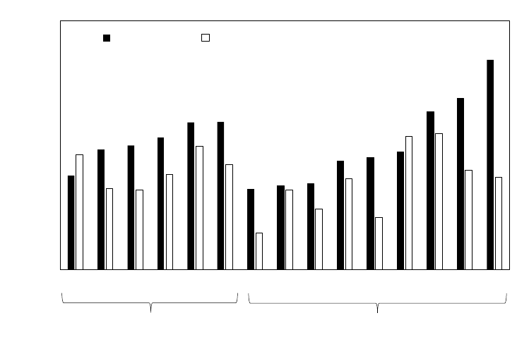
FIGURE 12. HMR borrower age at time of purchase, by LTV ≥90%

AT LU BE PT DE FR IE LV EE CY SI GR IT ES NL

Age of buyer (average 2004-08)

LTV<90 ltv>=90

No RRE boom-bust

RRE boom-bust

Source: HFCS.

The positive correlation between age and income also implies that more buyers are also

coming from higher-up the income distribution (Figure 13). In the majority of countries,

around 70% of borrowers come from the top two income quintiles in wave 2 up from

closer to 60% in wave 1 for many of these countries. In Germany, Estonia, Latvia, Austria

and Portugal, almost half of HMR mortgage borrowers are from the top 20% of the

income distribution in the period after 2010. This compares to 36% in Ireland and 28% in

Spain and Belgium. Borrowers in the bottom quintile of the income distribution account

for less than 5% of HMR mortgages in all countries after 2010, whereas prior to this the

percentage exceeded 10% in some countries (e.g. Germany and Netherlands).

FIGURE 13. HMR income distribution Borrowers 2006-09 vs. Borrowers 2010-13

0 20 40 60 80 100

percent

New loans for house purchase 2006-2009

0 20 40 60 80 100

percent

New loans for house purchase 2010-2013

Source: HFCS Wave 1 (top panel) and Wave 2. As income is only observed at each wave we restrict

comparisons to borrowers in the three years prior to each wave.

HMR versus Non-HMR property

One explanation for the change in borrower composition towards higher ages and

incomes that is pronounced in some of the countries is that it represents an increased

appetite for real assets at a time when the real return on deposits or other forms

of ﬁnancial assets is at an all-time low. Real estate may therefore represent a more

attractive investment, both in terms of an income stream and capital appreciation.

Similar behaviour was evident in some boom-bust countries before the bust, when a

combination of easy credit, low real interest rates, rising real house prices and favourable

tax treatment led to a large increase in buy-to-let investments.

Table 5 shows that

there has been a shift towards ownership of non-HMR real estate in some countries –

such as Germany, Netherlands, Belgium and (surprisingly) Spain. In France, on the other

hand, the increasing demand for real-estate assets is mainly evident in the substantial

increase in HMR home-ownership.

TABLE 5. HMR and other real estate ownership across countries & waves

HMR homeownership, %households Non-HMR real estate ownership, %households

Wave 1 Wave 2 Change Wave 1 Wave 2 Change

SK 89.9% 85.4% -4.5% CY 51.6% 46.0% -5.7%

CY 76.7% 73.5% -3.2% GR 37.9% 35.7% -2.2%

FI 69.2% 67.7% -1.5% IT 24.9% 23.1% -1.8%

PT 76.0% 74.7% -1.3% LU 28.2% 26.3% -1.8%

IT 68.7% 68.2% -0.5% AT 13.4% 12.1% -1.3%

GR 72.4% 72.1% -0.3% FR 24.7% 23.4% -1.3%

AT 47.7% 47.7% -0.1% FI 30.0% 30.5% 0.5%

DE 44.2% 44.3% 0.1% PT 29.1% 30.3% 1.2%

NL 57.1% 57.5% 0.4% NL 6.1% 8.1% 2.0%

ES 82.7% 83.1% 0.4% BE 16.4% 18.5% 2.1%

LU 67.1% 67.6% 0.5% DE 17.8% 20.2% 2.4%

BE 69.6% 70.3% 0.7% MT 31.2% 34.4% 3.2%

MT 77.7% 80.2% 2.5% SK 15.3% 19.4% 4.1%

FR 55.3% 58.7% 3.5% ES 36.2% 40.3% 4.2%

IE 70.5% PL 18.9%

SI 73.7% HU 23.0%

LV 76.0% IE 23.0%

EE 76.5% SI 30.6%

PL 77.4% EE 32.0%

HU 84.2% LV 39.1%

Source: HFCS waves 1 and 2. Country weights applied.

As we showed earlier, the headline ownership statistics hide considerable variation

in the age-proﬁle of real-estate ownership. In Figures 14 and 15 we show the rates of

HMR and other real estate ownership by decade of birth for those countries in Table 5

where we observe the largest changes between waves. Most notably in Germany, HMR

ownership has decreased for the youngest cohort (those born after 1980) while it has

substantially increased for the older cohorts (born between 1950 and 1970). In contrast,

in Belgium, the Netherlands, Spain and France households in the youngest cohort have

Lydon and O’Hanlon (2012) show that from 2002 to 2007, the share of buy-to-let loans

in Ireland increased more than ﬁve-fold, from less than 5% to over 25% of lending. When the

property market crashed, these loans proved to be ex-post highly risky for lenders, with over 37%

of balances in deep arrears at the trough of the crisis (June 2014), many of which were very long-

term loans (30+ years), often with interest-only repayment arrangements.

increased their HMR ownership. As for Non-HMR ownership, this has increased for all

cohorts in the depicted countries, including Germany between the two waves. This could

indicate that real estate is increasingly becoming attractive for investment rather than

just consumption purposes.

FIGURE 14. HMR ownership by decade born

10%

20%

30%

40%

50%

60%

70%

80%

90%

194019501960197019801990

% households in owner-occupied property

Decade born

HMR ownership - Belgium

Wave 1 Wave 2

10%

20%

30%

40%

50%

60%

70%

194019501960197019801990

% households in owner-occupied property

Decade born

HMR ownership - Germany

Wave 1 Wave 2

10%

20%

30%

40%

50%

60%

70%

80%

90%

100%

194019501960197019801990

% households in owner-occupied property

Decade born

HMR ownership - Spain

Wave 1 Wave 2

10%

20%

30%

40%

50%

60%

70%

80%

194019501960197019801990

% households in owner-occupied property

Decade born

HMR ownership - Netherlands

Wave 1 Wave 2

10%

20%

30%

40%

50%

60%

70%

80%

194019501960197019801990

% households in owner-occupied property

Decade born

HMR ownership - France

Wave 1 Wave 2

FIGURE 15. Other real estate ownership by decade born

10%

15%

20%

25%

194019501960197019801990

% households in owner-occupied property

Decade born

Ownership of other real estate - Belgium

Wave 1 Wave 2

10%

15%

20%

25%

30%

35%

194019501960197019801990

% households in owner-occupied property

Decade born

Ownership of other real estate - Germany

Wave 1 Wave 2

10%

20%

30%

40%

50%

60%

194019501960197019801990

% households in owner-occupied property

Decade born

Ownership of other real estate - Spain

Wave 1 Wave 2

10%

12%

194019501960197019801990

% households in owner-occupied property

Decade born

Ownership of other real estate - Netherlands

Wave 1 Wave 2

10%

15%

20%

25%

30%

35%

40%

194019501960197019801990

% households in owner-occupied property

Decade born

Ownership of other real estate - France

Wave 1 Wave 2

Source: HFCS Wave 1 and Wave 2. Note: scales differ by country.

5 Credit Constraints

The ﬁnancial instability consequences of a credit-driven boom-and-bust are generally

well understood. For example, Kelly and O’Malley (2016) show that, in a down-turn,

more leveraged borrowers and borrowers with heavier debt-service burdens tend to

be the most likely to experience repayment problems. The consequences of over-

indebtedness for the real economy have also been explored in Dynan (2012) and Mian

and Suﬁ (2015), who show how balance sheet rebuilding and credit constraints can drag

on household consumption after a credit bubble bursts. In this section, we use the HFCS

to analyse how the build-up of credit described in the previous section contributes to

households being credit constrained.

In the HFCS, a household is deﬁned as being credit constrained if it answers yes to

either of the two following questions: (1) “In the last three years, has any lender or

creditor turned down any request you [or someone in your household] made for credit,

or not given you as much credit as you applied for?”; (2) “In the last three years, did

you [or another member of your household] consider applying for a loan or credit but

then decided not to, thinking that the application would be rejected?”

We analyse the

incidence of credit constraints conditional on demanding credit in the ﬁrst place. That is,

in our regression sample a household has either had to have asked for credit and been

accepted or rejected, or not have asked for credit (but wanted it) for fear of rejection.

This naturally gives rise to potential selection bias issues, which should be borne in mind

when interpreting the results.

FIGURE 16. Credit constrained households and indebtedness

y = 0.2607x - 0.0626

R² = 0.6025

10%

15%

20%

25%

40% 50% 60% 70% 80% 90%

% credit constrained households

Current LTV, all HMR owners with a mortgage

Not conditioning on demanding credit

y = 0.638x - 0.2033

R² = 0.6225

10%

15%

20%

25%

30%

35%

40%

45%

50%

40% 50% 60% 70% 80% 90% 100%

% credit constrained households

Current LTV, all HMR owners with a mortgage

Conditional on demanding credit

Source: Wave 2 HFCS, 2014 for most countries. Charts show the country level mean of credit constrained

[0:1], as deﬁned in the text, and current LTV for HMR households with a mortgage.

Figure 16 provides graphical evidence at the country level on the relationship

between leverage and credit constraints. The charts show the percentage of HMR

mortgage households in each country that are credit constrained and the mean current

LTV for the same households. There is a positive correlation between leverage and

the prevalence of credit constraints, regardless of whether we condition on demanding

credit (right-hand side chart) or not, although the relationship is stronger in the

conditional group. However, the fact that there is a clear positive relationship for the

two groups gives some comfort that potential selection issues are unlikely to impact on

See Jappelli et al. (1998) for an early paper using self-reported credit constraints.

the substantive results, namely that higher leverage tends to be strongly correlated with

the incidence of credit constraints.

The country-level evidence in Figure 16 does not control for factors that might

be positively correlated with the likelihood of a household being credit constrained,

such as incomes or country-speciﬁc credit supply shocks. Therefore, we run a probit

model on the household level data where the dependent variable takes a value of one

if a household is credit constrained. The marginal effects from the probit model, in

Table 6, conﬁrm the country-level patterns reported above: more highly leveraged

households and/or households with larger debt-repayment burdens are much more

likely to experience credit constraints, controlling for income and other factors, including

country ﬁxed effects.

To allow for any additional effects common to boom-bust countries, we allow

coefﬁcients on leverage and debt service to vary by boom-bust/non boom-bust

countries. We also employ piece-wise speciﬁcations (columns (2) and (4)) to allow the

effects of indebtedness/debt-service to be non-linear. These speciﬁcations conﬁrm that

the effects of indebtedness on the probability of being credit constrained are indeed

stronger for boom-bust countries, and highly non-linear. The average marginal effects

can be interpreted as additive. Take column 1, Table 6 as an example. Going from a

very low LTV to high LTV (100%) increases the likelihood of being credit constrained

by 2.4%. In boom-bust countries, the marginal effect is almost doubled (4.35% = 2.4%

+ 1.95%) . Similarly, a higher income reduces the likelihood of being credit constrained

by 9.6%, but the income effect is almost a third lower in boom-bust countries (6.8% =

9.6%-2.8%). The impact of LTV on the likelihood of being credit constrained is non-

linear. For example, in column (2) households in negative equity in boom-bust countries

(LTV>100) are 6.6% more likely to experience credit constraints (versus a sample mean

of 25.8%), compared with a ﬁgure of 1.75% for negative equity households in non boom-

bust countries (sample mean of 14.5%). Similar effects are observed when we look at the

debt-service ratio instead of LTV.

TABLE 6. Credit constraints regression results

Marginal effects from a probit model (1) (2) (3) (4)

Log income -0.0958*** -0.0957*** -0.0922*** -0.08912***

(0.00403) (0.00403) (0.00487) (0.00461)

Log income × boom-bust 0.0279*** 0.0276*** 0.0387*** 0.0353***

(0.0059) (0.0059) (0.0074) (0.0070)

Current LTV 0.0243***

(0.00502)

Current LTV × boom-bust 0.01958***

(0.0071)

LTV<75 [Omitted]

LTV 75-100 -0.00919

(0.00653)

LTV 75-100 × boom-bust -0.00411

(0.0110)

LTV>100 0.0175***

(0.0077)

LTV>100 × boom-bust 0.0668***

(0.0106)

Debt-service ratio 0.0843***

(0.01481)

Debt-service ratio × boom-bust -0.0177

(0.0240)

Debt-service ratio < 30% of income [Omitted]

Debt-service ratio 30-39% 0.0410***

(0.0088)

Debt-service ratio 30-39% × boom-bust 0.0247**

(0.0142)

Debt-service ratio ≥40% 0.0740***

(0.0917)

Debt-service ratio ≥40% × boom-bust -0.0431***

(0.0147)

Demographic controls Yes Yes Yes Yes

Country Fixed Effects Yes Yes Yes Yes

E[Credit-Constrained, non boom-bust] 14.5% 14.5% 14.5% 14.5%

E[Credit-Constrained, boom-bust] 25.8% 25.8% 25.8% 25.8%

Observations 39,778 39,874 39,109 39,109

R2 0.11 0.11 0.11 0.11

Source: HFCS waves 1 and 2, households with a HMR (‘household main residence’) mortgage. Conditional on

HFCS deﬁnition of being credit constrained as deﬁned in the text. Demographic and other controls include age,

education, gender, survey wave and country ﬁxed effects. The debt service ratio is as a percentage of gross

household income. The table displays average marginal effects from a probit regression.

Endogeneity problems such as omitted variable bias (unobserved heterogeneity

leading to credit constraints) and reverse causality (for example, if households prioritise

debt repayments and reduce LTV to avoid future credit constraints) makes causal

interpretation of the coefﬁcients difﬁcult. We therefore estimate a differenced model

where the dependent variable is equal to one if a household becomes credit constrained

between the two survey waves. In order to become credit constrained a household has

to have demanded credit in both waves, but only be rejected in wave 2 of the HFCS.

Conditioning on demanding credit, combined with the fact that only a subset of countries

have a panel element (Germany, Cyprus, Belgium, Spain, Malta and Netherlands) reduces

our regression sample. Our primary focus here is comparing the signs and signiﬁcance of

the coefﬁcients on the variable of interest with the earlier cross-section results. Table 7

shows the results. As we are only using a subset of countries, we do not include a boom-

bust interaction term.

TABLE 7. Probability of becoming credit constrained regression results

Marginal effects from a probit model (1) (2) (3) (4) (5) (6)

∆ income -0.0515*** -0.0491*** -0.0495*** -0.0427*** -0.0343** -0.0452***

(0.0121) (0.0121) (0.0120) (0.0135) (0.0124) (0.0162)

Current LTV 0.0431***

(0.0093)

LTV<75 [Omitted]

LTV 75-100 0.0409***

(0.0133)

LTV>100 0.0700***

(0.0120)

∆ LTV 0.0698***

(0.0102)

Current debt-service ratio 0.0720***

(0.0161)

Debt-service ratio < 30% [Omitted]

Debt-service ratio 30-39% 0.0403**

(0.0151)

Debt-service ratio ≥40% 0.0561***

(0.0131)

∆ Debt-service ratio 0.0629**

(0.0240)

Demographics Yes Yes Yes Yes Yes Yes

Country Fixed Effects Yes Yes Yes Yes Yes Yes

E[Become CC] 8.0% 8.0% 8.0% 8.0% 8.0% 8.0%

Observations 3,350 3,350 3,345 3,290 3,350 3,222

R-squared 0.067 0.075 0.078 0.069 0.067 0.069

Source: HFCS waves 1 and 2, only countries with panel component. Demographic controls are age, age-squared

and change in household size.The table displays average marginal effects from a probit regression.

The key result is that all of the earlier results on income, leverage, repayment burden

and non-linear effects also hold in the ‘differenced’ sample. In fact, if anything the

impact of all of these factors has increased, relative to the sample mean outcome. For

example, a household in negative equity (LTV>100) in wave 2 is far more likely to be

credit constrained versus a household with an LTV under 75%, controlling for income

shocks, demographics and country ﬁxed effects. Similar marginal effects are evident for

the high debt-service households. We also estimate speciﬁcations where the current

LTV and debt-service ratio is instrumented with the lag and the results are unchanged.

6 Conclusion

Using cross-country micro data, our paper provides evidence of the evolution of

institutional features and of household behaviour with respect to real estate investment

in boom-bust and non-boom-bust countries over time. For countries that experienced a

real estate boom-and-bust there is evidence of a deterioration of credit standards before

the Financial Crisis, with higher LTVs, LTIs and signiﬁcantly longer loan terms. Borrowers

with high origin LTVs also exhibit higher debt service burdens, particularly among lower

income (often younger) households. Credit standards have become more restrictive

after the crisis, in many cases anticipating the introduction of explicit borrower based

macroprudential limits.

In contrast, the non-boom-bust group did not experience a similar easing of credit

standards before the crisis or during the more recent period of historically low interest

rates, even as house prices have been rising in some of these countries.

Turning to the real effects of over-indebtedness, we show that having too much debt

is positively correlated with households being credit-constrained, exacerbating credit-

driven boom-bust dynamics. Speciﬁcally, we should that borrowers with high levels of

leverage are more likely to become credit constrained, even after controlling for income

shocks, demographics and country ﬁxed effects.

The typical borrower has changed since the Financial Crisis in all countries.

Particularly older and more afﬂuent households invest more in real estate, both in main

residence and buy-to-let. This change may be driven by a portfolio shift and a search for

yield that traditional low-risk ﬁnancial assets do not give in times of low interest rates.

In boom-bust countries, this compositional shift may reﬂect tighter lending standards, a

fall in incomes and delayed labour market participation by young households. The social

implications are the same for both groups: younger households need to save longer in

order to afford higher house prices and make down payments.

Our analysis has the following policy implications: given that monetary policy targets

the Euro area as a whole, the high degree of heterogeneity in lending standards and

borrower characteristics reveals the important role of macroprudential responses to

risks in the ﬁnancial system, in addition to micro-prudential policies. In this respect, the

use of high quality micro data on households’ balance sheets, including indebtedness,

ﬁnancial and real assets is a useful tool for the assessment of micro and macro prudential

risk stemming from the household sector. Using such data can potentially uncover the

build-up of pockets of risk within and across countries. Furthermore, it can uncover

important societal changes in borrower composition: macroprudential policies are not

implemented in a vacuum and policy makers therefore need to be aware of any such

changes.

References

Albacete, N., Eidenberger, J., Krenn, G., Lindner, P., and Sigmund, M. (2014). Risk-

bearing capacity of households–linking micro-level data to the macroprudential

toolkit. Financial Stability Report, 27:95–110.

Albacete, N., Fessler, P., and Lindner, P. (2016). The distribution of residential property

price changes across homeowners and its implications for ﬁnancial stability in Austria.

Financial Stability Report, 31:62–81.

Ampudia, M., Pavlickova, A., Slacalek, J., and Vogel, E. (2016). Household heterogeneity

in the euro area since the onset of the Great Recession. Journal of Policy Modeling,

38(1):181–197.

Behn, M., Gross, M., and Peltonen, T. A. (2016). Assessing the costs and beneﬁts of

capital-based macroprudential policy.

Blanchard, O. (2007). Adjustment within the euro. The difﬁcult case of Portugal.

Portuguese Economic Journal, 6(1):1–21.

Byrne, D., Kelly, R., and O’Toole, C. (2017). How does monetary policy pass-through

affect mortgage default? Evidence from the Irish mortgage market. Central Bank of

Ireland, Research Technical Paper No. 04/RT/17.

CBI (2016). Review of residential mortgage lending requirements. Central Bank of Ireland

Review.

Cerutti, E., Claessens, S., and Laeven, M. L. (2015). The use and effectiveness of

macroprudential policies: new evidence. Number 15-61. International Monetary Fund.

Claessens, S. (2015). An overview of macroprudential policy tools. Annual Review of

Financial Economics.

Claessens, S., Kose, M. A., and Terrones, M. E. (2009). What happens during recessions,

crunches and busts? Economic Policy, 24(60):653–700.

Coates, D., Lydon, R., and McCarthy, Y. (2015). House price volatility: the role of different

buyer types. Central Bank of Ireland, Economic Letter Series 02-EL-2015.

Costa, S. and Farinha, L. (2012). Households’ indebtedness: A microeconomic analysis

based on the results of the households’ ﬁnancial and consumption survey. Financial

stability report. Banco de Portugal. May.

Crowe, C., Dell Ariccia, G., Igan, D., and Rabanal, P. (2013). How to deal with real estate

booms: Lessons from country experiences. Journal of Financial Stability, 9(3):300–319.

Cussen, M., O’Brien, M., Onorante, L., and O’Reilly, G. (2015). Assessing the impact

of macroprudential measures. Central Bank of Ireland, Economic Letter Series 03-EL-

2015.

de Caju, P. (2016). Survey evidence of pockets of risk in the Belgian mortgage market: A

micro analysis based on HFCS data. Mimeo.

Dynan, K. (2012). Is a household debt overhang holding back consumption? Brookings

Papers on Economic Activity, pages 299–362.

ECB (2013). The eurosystem Household Finance and Consumption Survey – Results

from the ﬁrst wave. ECB Statistics Paper Series, No. 2.

ECB (2016). The eurosystem Household Finance and Consumption Survey – Results

from the second wave. ECB Statistics Paper Series, No. 18.

ESRB (2015). Report on residential real estate and ﬁnancial stability in the EU. ESRB

Report.

ESRB (2016). Vulnerabilities in the eu residential real estate sector. ESRB 2016.

Fagan, G. and Gaspar, V. (2005). Adjusting to the euro area: some issues inspired by the

Portuguese experience. In A Conference organized by the ECB on “What effects is EMU

having on the euro area and its member countries”, pages 16–37.

Hartmann, P. (2015). Real estate markets and macroprudential policy in Europe. Journal

of Money, Credit and Banking, 47(S1):69–80.

Jappelli, T., Pischke, J.-S., and Souleles, N. S. (1998). Testing for liquidity constraints in

euler equations with complementary data sources. Review of Economics and statistics,

80(2):251–262.

Kelly, J. and Lydon, R. (2017). Home purchases, downpayments and savings. Central Bank

of Ireland, Economic Letter Series 02-EL-2017.

Kelly, R., McCann, F., and O Toole, C. (2015). Credit conditions, macroprudential policy

and house prices. Central Bank of Ireland, Research Technical Paper No. 06/RT/15, 6.

Kelly, R. and O’Malley, T. (2016). The good, the bad and the impaired: A credit risk model

of the irish mortgage market. Journal of Financial Stability, 22:1–9.

Kinghan, C., Lyons, P., and McCarthy, Y. (2017). Macroprudential Measures and Irish

Mortgage Lending:Insights from H1 2017. Central Bank of Ireland, Economic Letter

Series 13-EL-2017.

Laeven, L. and Popov, A. (2017). Waking up from the American dream: on the experience

of young Americans during the housing boom of the 2000s. Journal of Money, Credit and

Banking, 49(5):861–895.

Le Blanc, J. (2016). Household Saving Behaviour in Ireland. Central Bank of Ireland,

Economic Letter Series 05-EL-2016.

Lydon, R. and McCann, F. (2017). The income distribution and the Irish mortgage market.

Central Bank of Ireland, Economic Letter Series 05-EL-2017.

Marek, P. (2017). Homeownership Rates of young households in Germany. Technical

report.

Mian, A. and Suﬁ, A. (2015). House of debt: How they (and you) caused the Great Recession,

and how we can prevent it from happening again. University of Chicago Press.

Reis, R. (2013). The Portuguese Slump and Crash and the Euro Crisis. Brookings Papers

on Economic Activity, page 172.

Room, T. and Merikall, J. (2017). The ﬁnancial fragility of Estonian households: Evidence

from stress tests on the HFCS microdata. Bank of Estonia, Working Paper.

Thebault, L. (2017). The “v” in ltv and why it matters. EMF Hypostat.

Appendix charts

FIGURE 17. Cross-country house price trends in the HFCS data

100

150

200

100

150

200

100

150

200

1995 2000 2005 2010 2015 1995 2000 2005 2010 2015

1995 2000 2005 2010 2015

EE IE GR

ES IT NL

HFCS OECD

100

150

100

150

100

150

1995 2000 2005 2010 20151995 2000 2005 2010 2015

1995 2000 2005 2010 2015

BE DE FR

LU AT PT

HFCS data OECD

Source: HFCS, waves 1 and 2.

We thank Gabriel Fagan and Fergal McCann and participants at the March 2017 HFCN meeting, the June 2017

meeting of the Heads of Research of the ESCB, Irish Economics Association Annual Conference, International

Finance and Banking Society (Porto, 2018) and Central Bank of Ireland Economic Seminars for comments on

earlier drafts that greatly improved the paper. The views in this paper are those of the authors only and not of

the Central Bank of Ireland, the Deutsche Bundesbank or the ESCB.

Jane Kelly

Central Bank of Ireland, Dublin, Ireland; e-mail: [email protected]

Julia Le Blanc

Deutsche Bundesbank, Frankfurt am Main, Germany; e-mail: julia.le.blanc@bundesbank.de

Reamonn Lydon (corresponding author)

Central Bank of Ireland, Dublin, Ireland; e-mail: reamonn.ly[email protected]

Imprint and acknowlegements

Postal address 60640 Frankfurt am Main, Germany

Telephone +49 69 1344 0

Website www.esrb.europa.eu

source is acknowledged.

Note:

The views expressed in ESRB Working Papers are those of the authors and do not necessarily reflect

the official stance of the ESRB, its member institutions, or the institutions to which the authors are

affiliated.

ISSN 2467-0677 (pdf)

ISBN 978-92-9472-073-3 (pdf)

DOI 10.2849/694 (pdf)

EU catalogue No DT-AD-19-001-EN-N (pdf)