Data Reduction, Summary, and Presentation

Travel Time Data Collection Handbook 7-1

7 DATA REDUCTION, SUMMARY, AND PRESENTATION

This chapter provides guidance on the reduction, summary, and presentation of travel time data.

Chapters 3 through 5 contained specific data reduction and quality control procedures for each data

collection technique. The procedures in earlier chapters were aimed at producing a common travel

time format for each predefined roadway segment or link. The methods described in this chapter can

then be used to further reduce, summarize, and/or present this travel time data. Many examples of

tabular and graphical summaries of travel time data are provided at the end of the chapter.

7.1 Data Reduction

This section contains a discussion on the purposes and methods used to reduce and/or aggregate

travel time data. It is assumed that appropriate data reduction and quality control measures have

been applied for the specific data collection technique, and that the travel time data are in an

individual link format (i.e., data contains valid individual travel times for each predefined link or

segment length). Quality control procedures for each data collection technique were included in

Chapters 3 through 6. The purpose of data reduction can be two-fold:

• reduce the number of data records by eliminating invalid data; or

• produce summary data and statistics at different aggregation levels for various

applications.

Quality control measures applied to the data immediately after data collection should have identified

data errors or invalid data. However, statistical quality control checks can be performed at this point

to identify any remaining problems with data integrity. Statistical quality control procedures are

available in some spreadsheet and database software programs and in nearly all statistical analysis

software packages. Readers interested in statistical quality control procedures should consult a

specialized statistics text.

In most cases, data reduction will be necessary to summarize or aggregate the link travel time data

to a format usable in many analyses. Travel times from individual runs should be averaged to

produce mean or average travel times for the peak hour or peak period. Individual travel times from

license plate matching should be averaged to produce average travel times and speeds for 15- or 30-

minute time periods or greater. Typical summary statistics computed with link travel time data

include:

• Mean or average travel time, speed, and delay - These statistics provide

information about the typical traffic conditions during the time period of interest.

Means or averages can be computed for any time period desired, including but not

limited to 15-, 30-, or 60-minute, peak hour, and peak period (Equations 7-1, 7-2, and

7-3). The selected time period typically corresponds to analysis needs and available

Average Travel Time, t '

i'1

Space&Mean (Harmonic) Speed, v

SMS

distance traveled

avg. travel time

n×d

Average Vehicle

(or Person) Delay

' (t & t

delay

) × V (or P) '

delay

& s* × V (or P)

CHAPTER 7 - DATA REDUCTION, SUMMARY, AND PRESENTATION

7-2 Travel Time Data Collection Handbook

(7-1)

(7-2)

(7-3)

sample sizes. For example, travel time data collected with license plate matching or

ITS probe vehicle techniques can be summarized for shorter time periods because of

the typically larger sample sizes. Travel time data collected using test vehicle

techniques are generally aggregated to the peak hour or peak period because of

smaller sample sizes (less than 10 runs per time period per direction).

where: = average travel time for time period of interest

t = average travel time for i-th run or vehicle

n = total number of travel times

d = vehicle distance traveled or segment length

where: t = threshold travel time at which delay occurs

delay

s = threshold speed at which delay occurs

delay

V = vehicle volume for the time period of interest

P = person volume for the time period of interest

A more general form for an average space mean speed is presented in Equation 7-4

(1,2). This equation can be used when a different number of travel time observations

exist for numerous sequential roadway links. For example, an average corridor travel

speed is obtained from Equation 7-4 by computing the average travel time for each

roadway link, then weighting each link travel time by the respective number of travel

time observations. This approach, which weights each link travel time, has been

suggested by Quiroga and Bullock as a better estimator of average corridor travel

speeds. An alternative to average travel speed is the average median travel speed as

shown in Equation 7-5.

Average Space

Mean Speed, u

i'1

j'1

Median Speed, u

i'1

standard deviation, s '

i'1

& t)

n & 1

CHAPTER 7 - DATA REDUCTION, SUMMARY, AND PRESENTATION

Travel Time Data Collection Handbook 7-3

(7-4)

(7-5)

(7-6)

where: = average space mean (harmonic) speed for total length L

L = total length of roadway for calculation of average speed

= total travel time for entire length of roadway L

L = length of roadway link i

m = total number of travel time observations for each link i

u = travel speed for roadway link i and observation j

where: = median travel time associated with link i

= median speed associated with link i

• Standard deviation (or coefficient of variation) of speed and travel time - These

statistics provide information about the variability of traffic conditions throughout

the time period of interest. The standard deviation and coefficient of variation are

statistical measures of variability and are calculated using Equations 7-6 and 7-7,

respectively.

coefficient of variation, c.v. '

acceleration noise, a.n. '

i'1

& a)

n & 1

CHAPTER 7 - DATA REDUCTION, SUMMARY, AND PRESENTATION

7-4 Travel Time Data Collection Handbook

(7-7)

(7-8)

• Acceleration noise (i.e., standard deviation of acceleration) - Acceleration noise

(Equation 7-8) measures the fluctuation of speed for a typical vehicle and can only

be collected with a properly instrumented test or ITS probe vehicle. The desired

instrumentation should be capable of providing nearly second-by-second speeds of

a vehicle traveling in the traffic stream. Acceleration noise measures the “stop-and-

go” nature of congested traffic conditions or poorly timed traffic signals on arterial

streets. Previous studies have linked acceleration noise to a number of dependent

variables, such as accident rate, fuel consumption and mobile source emissions (3).

• Level of service (LOS) based on speed or travel time criteria - The 1994 Highway

Capacity Manual (HCM) uses average speed as an LOS criteria for arterial streets and

the year 2000 HCM is oriented toward similar speed/travel time criteria for most

analysis modules.

The aggregation and summarization of travel time data are fairly straightforward using current

computer tools. Computer spreadsheets, databases, GIS, and statistical analysis software packages

can immensely simplify the data reduction and summarization process. In most cases, data reduction

and summarization consists of either averaging or summing travel time or speed data. However,

several notes of caution for data reduction are provided below:

• Ensure that space-mean speeds are calculated - Space-mean speeds are associated

with a given length of roadway and are calculated using Equation 7-2. Time-mean

speeds are associated with a specified point along the roadway and are calculated by

simply averaging spot speeds. Chapter 1 and Table 1-1 contains a specific example

illustrating the proper calculation of space-mean speeds.

• Use vehicle or person volume to weight average speeds - Travel time and speed

data collected for a specific roadway segment also has a vehicle or person volume

associated with that segment. This volume quantifies the number of vehicles or

average weighted speed, spd

' (spd

×V

) % (spd

×V

) % . . . % (spd

×V

)

average corridor travel time, t

' t

% t

% . . . % t

CHAPTER 7 - DATA REDUCTION, SUMMARY, AND PRESENTATION

Travel Time Data Collection Handbook 7-5

(7-9)

(7-10)

persons traveling at the corresponding average speed. This vehicle or person volume

should be used to weight speeds when combining or averaging speeds for different

segments or corridors (see Equation 7-9).

• Aggregating travel times for a long corridor - Consider an analysis that requires

an average overall travel time for a 30-km roadway corridor. The average overall

travel time can be computed by simply summing the individual link or segment travel

times (Equation 7-10).

However, if the overall corridor travel time is greater than the applicable time period

in which the travel times were collected, Equation 7-10 does not provide an accurate

overall corridor travel time. For example, assume that average link travel times have

been collected between 7:00 and 7:30 a.m. (30-minute time period), yet it required

45 minutes (as estimated by Equation 7-10) to traverse the entire 30-km length of the

corridor (see Table 7-1, Scenario 1). In this scenario, at least 15 minutes of the

“corridor trip” could have occurred outside of the time period in which there is valid

travel time data (i.e., 7:00 to 7:30 a.m.). Three solutions exist for this dilemma:

1. Avoid the problem by equipping a test vehicle to perform travel time runs

along the entire length of the corridor. Simply average the overall corridor

travel time from each test vehicle run.

2. Increase the length of the analysis time period so that it is at least as long as

the total time required to traverse the entire corridor (Table 7-1, Scenario 2).

In this scenario, travel times were averaged from 7:00 to 8:00 a.m. so that we

could simply sum the link travel times for an overall corridor travel time.

3. Collect or obtain data for several small sequential time periods and apply the

average link travel time from the correspondingly correct time period (Table

7-1, Scenario 3). In this scenario, average travel times were computed from

7:30 to 8:00 a.m. If we assume that 20 minutes of the estimated 45-minute

“corridor trip” occurred in the 7:00 to 7:30 a.m. time period, then we can

determine how many roadway segments were traversed during that time

period. We can then apply the travel times from the next time period, 7:30

to 8:00 a.m., for the remainder of the roadway segments in the corridor.

CHAPTER 7 - DATA REDUCTION, SUMMARY, AND PRESENTATION

7-6 Travel Time Data Collection Handbook

Table 7-1. Corridor Travel Time Aggregation Example

Corridor

Segment

Travel Time (min:sec)

Scenario 1 Scenario 2 Scenario 3

7:00 to 7:30 a.m. 7:00 to 8:00 a.m.

7:00 to 7:30 a.m. 7:30 to 8:00 a.m.

1 6:00 5:30 6:00 5:00

2 5:20 4:40 5:20 4:00

3 4:40 4:00 4:40 3:20

4 5:40 5:20 5:40 5:00

5 6:00 5:40 6:00 5:20

6 4:30 4:00 4:30 3:30

7 3:40 3:40 3:40 3:40

8 4:00 4:00 4:00 4:00

9 2:30 2:30 2:30 2:30

10 2:20 2:00 2:20 1:40

Corridor 45:00 41:20 43:00

Travel

Time

(but analysis period (okay since analysis (okay since travel times from corresponding time

only 30 minutes) period is 60 minutes) period are used)

CHAPTER 7 - DATA REDUCTION, SUMMARY, AND PRESENTATION

Travel Time Data Collection Handbook 7-7

7.2 Overview of Travel Time Data Applications

Travel time data are collected for a variety of applications and analyses. This section provides a brief

overview of common applications of travel time data. The reader is encouraged to review the

companion handbook on travel time applications. At press time, this guidance manual on

applications of travel time data travel time was being prepared for FHWA by the Texas

Transportation Institute.

Travel time data are the raw element for a number of performance measures that permeate many

transportation analyses. Examples of travel-time based quantities or measures include the following:

• door-to-door travel time;

• travel time reliability/variability (i.e., standard deviations or confidence intervals);

• average speed;

• person or vehicle delay (as compared to some delay threshold);

• delay rate, relative delay rate, or delay ratio;

• speed of person movement (requires estimate of person volumes);

• travel time or congestion indices for corridors or networks; and

• accessibility to activities or opportunities (e.g., percent of population within 20

minutes of jobs, hospital, etc.).

Travel time-based measures can be used in transportation planning, design and operations, and

evaluation. Examples of planning and design applications include:

• Develop transportation policies and programs - may rely on current and projected

trends in travel time-based performance measures;

• Perform needs studies or assessments - may use travel time-based measures to assess

transportation deficiencies and potential improvements;

• Rank and prioritize transportation improvements - may use numerical magnitude of

travel time-based measures to set funding or programming priorities;

• Evaluate transportation improvement strategies - compare a number of possible

alternatives using a set of travel time-based measures;

• Input/calibration of planning models - uses base data such as travel time or speed to

compare simulated data to existing conditions, and projecting future scenarios; and

• Calculate road user costs for economic analyses - uses basic data as inputs to

economic models that estimate costs and benefits.

CHAPTER 7 - DATA REDUCTION, SUMMARY, AND PRESENTATION

7-8 Travel Time Data Collection Handbook

Examples of operational applications include:

• Develop historical database of traffic conditions - an historical database of travel

times and speeds can be used in numerous ITS applications;

• Input/calibration of traffic models - uses detailed data for model calibration relating

to microscopic traffic operations, fuel consumption, mobile source emissions;

• Real-time traffic control - uses travel time and speed to operate dynamic message and

lane assignment signs, ramp metering, and traffic signal control;

• Route guidance and navigation - provides travel time information and alternative

routes based on current or historical databases;

• Traveler information - provides up-to-date travel time and speed information to the

commuting public; and

• Incident detection - uses changes or differences in current travel time or speed as

compared to historical databases.

Examples of evaluation applications include:

• Establish/monitor congestion trends - collect and develop historical data for trend

analyses;

• Congestion management/performance measurement - tracking trends over time of

travel time-based measures, attempt to develop cause-and-effect relationships;

• Identify congestion locations or bottlenecks - uses travel time data in combination

with geometric or signal information to identify problems and potential solutions;

• Measure effectiveness and benefits of improvements - use before-and-after travel time

data to gauge the effects of transportation improvements;

• Communicate information to the public - use non-technical travel time-based

measures to communicate traffic conditions and trends to the general public; and

• Research and development - uses travel time data for a wide variety of research

applications.

CHAPTER 7 - DATA REDUCTION, SUMMARY, AND PRESENTATION

Travel Time Data Collection Handbook 7-9

7.3 Understanding Your Audience for Travel Time Summaries

One of the first principles taught in most technical writing courses is the importance of

understanding your audience. This same principle also applies to tabular and graphical data

summaries. These data summaries often serve as the only interpretation of extensive data collection

efforts for a wide variety of audiences. The manner in which data are presented, as well as the actual

data itself, is critical for effectively communicating the results of travel time collection activities.

The intended audience(s) for data summaries affects several aspects:

• Underlying message or theme of the summary - The intended audience directly

influences the underlying message or theme of the summary. For example, a mayor

of a large city is likely more interested in regional travel time and speed trends and

less interested in the number of stops for a particular travel time run. Conversely, a

city signal technician is likely more interested in the number and location of stops

along an arterial street.

• Manner of presentation (e.g., table versus graph/chart) - Concise, easy-to-

understand graphs or charts are best suited to non-technical audiences, whereas these

concise summaries may not contain enough information for detail-oriented, technical

audiences.

• Use of technical language/terminology - If decision-makers or elected officials will

utilize data summaries, technical language should be avoided if possible. At a

minimum, technical terms should be defined for unfamiliar readers.

• Level of detail - The level of detail should be appropriate for the intended audiences.

If a wide variety of readers is expected, different types of summaries should be

provided. Technical appendices can be provided for data collection details, and an

executive summary can be used to present the major findings of the study in

graphical or brief tabular formats.

7.4 Presenting Dimensions of Congestion with Travel Time and Speed Data

Travel time and speed data are often used to identify and evaluate traffic congestion patterns and

trends. It is important to note that traffic congestion has several “dimensions,” and that data

summaries should be designed to represent these four major dimensions (4):

• Duration - amount of time roadway facilities are congested;

• Extent - number of people affected or the geographic distribution;

• Intensity - level or total amount of congestion; and,

• Reliability - variation in the amount of congestion.

CHAPTER 7 - DATA REDUCTION, SUMMARY, AND PRESENTATION

7-10 Travel Time Data Collection Handbook

These dimensions of congestion can be represented with a number of travel time/speed measures,

depending upon the system component as shown in Table 7-2.

Table 7-2. Measures and Summaries to Display the Dimensions of Congestion

Congestion Aspect

System Type

Single Roadway Corridor Areawide Network

Duration (i.e., amount

of time system is

congested)

Hours facility operates Hours facility operates Set of travel time

below acceptable speed below acceptable speed contour maps;

“bandwidth” maps

showing amount of

congested time for

system sections

Extent (i.e., number of

people affected or

geographic distribution)

percent or amount of percent of VMT or PMT percent of trips in

congested VMT or PMT; in congestion; percent or congestion; person-km

percent or lane-km of lane-km of congested or person-hours of

congested road road congestion; percent or

lane-km of congested

roadway

Intensity (i.e., level or

total amount of

congestion)

Travel speed or rate; Average speed or travel Accessibility; total delay

delay rate; relative delay rate; delay per PMT; in person-hours; delay

rate; minute-km; lane-km delay ratio per person; delay per

hours PMT

Reliability or

Variability (i.e.,

variation in the amount

of congestion)

Average travel rate or Average travel rate or Travel time contour

speed + standard speed + standard maps with variation

deviation; delay + deviation; delay + lines; average travel/time

standard deviation standard deviation + standard deviation;

delay + standard

deviation

Notes: adapted from reference (4)

VMT—vehicle-miles of travel; PMT—person-miles of travel

CHAPTER 7 - DATA REDUCTION, SUMMARY, AND PRESENTATION

Travel Time Data Collection Handbook 7-11

7.5 Examples of Data Summaries

Tabular summaries contain numerical values in a row or column format, whereas graphical

summaries provide information in the form of a chart, graph, or picture. The choice of a tabular or

graphical summary depends upon the intended audience and the desired message. In general, tabular

summaries are best for presenting large amounts of data with some level of detail. Graphical

summaries are best suited to presenting relatively small amounts of easily understandable data.

Further, graphical summaries allow the viewer to quickly recognize trends and relative comparisons

of data with the visual presentation. Depending upon the level of detail, tabular summaries may take

longer to interpret than comparable graphical summaries. Also, technical audiences are generally

more effective at interpreting tabular summaries because of their numeric orientation and format.

Travel time data summaries may be provided at several levels of detail:

• Run summary - summarizes data on a specific travel time run, and typically includes

elapsed time and speed between checkpoints, causes of intermediate delay, and time

spent in different speed ranges. Run summaries are useful in performing quality

control on data collection efforts and diagnosing traffic operations problems at a

detailed scale.

• Aggregated run summary - aggregates data for several travel time runs or vehicles

along a single route, and typically includes average travel times and speeds between

checkpoints and totals for delay. Aggregated run summaries provide average

statistics for individual routes segments and are useful for a number of applications.

Data collected from license plate matching includes average travel times and speeds

for predefined roadway segments.

• Corridor or route summary - summarizes data for a corridor or route of

consequential length, and includes average travel times, speeds, and delays. Corridor

or route summaries are useful for large scale comparisons of traffic conditions and

for providing information to non-technical audiences.

• Functional classification summary - summarizes data for all roadways within

defined functional classifications (see Chapter 2), and includes average travel times,

speeds, and delays. Functional class summaries are also useful at a macroscopic

level for long range planning and time series trends.

• Other summaries - includes activity center summaries, travel time contours,

accessibility plots, and other types of summaries not fitting neatly into the above

categories. These types of summaries are more “system-oriented” than other

summaries and help to identify the system conditions and the system effects of

various transportation improvements.

CHAPTER 7 - DATA REDUCTION, SUMMARY, AND PRESENTATION

7-12 Travel Time Data Collection Handbook

The remainder of this chapter contains examples of these summaries with an interpretation of key

features. These examples are a representative sample of travel time data summaries that have been

used by transportation agencies. These examples are not a comprehensive inventory of all possible

summaries. Two other references (4,5) contain several additional examples of tabular and graphical

travel time data summaries. The figures and tables shown throughout this chapter are intended to

provide the user of this handbook with examples from previous studies, with the intent of aiding the

reader in identifying summaries applicable to their users and uses.

7.5.1 Run Summaries

A run summary includes data that have been collected during a specific travel time run, including

elapsed time and speed between checkpoints, causes of intermediate delay, and time spent in

different speed ranges. The run summaries are most common for test vehicle methods in which the

vehicle is instrumented and data can be frequently collected at intermediate locations. Run

summaries provide the finest level of detail for a travel time run, thereby providing a useful tool for

performing quality control or diagnosing traffic operations problems.

Figures 7-1 and 7-2 show a run summary for Corinth/Lancaster Street in Dallas. The travel time and

speed data shown in these figures were collected using the test vehicle method with an electronic

DMI (see Chapter 3). The speed profile in Figure 7-1 illustrates the speed of the test vehicle

throughout the entire length of the travel time run. Stops at intersections or mid-block speed

reductions are clearly denoted by “dips” in the speed profile. Speed profiles such as Figure 7-1

provide useful information at a glance on signal coordination and progression. Also, note that the

speed profile in Figure 7-1 is distance-based (i.e., x-axis is in distance units). A time-based speed

profile shows more information about the duration of stops, but systematic identification of cross

streets on a graph may be difficult. Graphing functions in most computer spreadsheets simplify the

task of producing distance-time, speed-distance, or acceleration-distance profiles. Software macros

also simplify the calculation of control delay, stopped delay, and other measures of effectiveness (6).

Figure 7-2 contains a tabular summary of the same travel time run illustrated in Figure 7-1. The

tabular summary in Figure 7-2 includes intermediate and cumulative distances, travel times, and

average speeds. This type of summary typically includes summary information on the cause and

magnitude of stops or traffic disruptions experienced during the travel time run. The tabular

summary in Figure 7-2 also contains information about the percent time spent in different speed

ranges and the level of service for Highway Capacity Manual calculations.

For less automated test vehicle methods, travel times and speeds may only be available at selected

intermediate checkpoints. Figure 7-3 illustrates the display of travel time, speed, and delay for a

given travel time run. Note that less detail is available for the speed profile and that only average

speeds are known between intermediate checkpoints. Table 7-3 contains an example of a tabular run

summary of travel times, speeds, and delays between intermediate checkpoints.

CHAPTER 7 - DATA REDUCTION, SUMMARY, AND PRESENTATION

Travel Time Data Collection Handbook 7-15

Average Speed

Between Intersections

(km/h)

Cumulative

Travel Time (min)

Source: adapted from reference (8)

Figure 7-3. Example Summary of Travel Time, Speed, and Delay Information

for an Arterial Street

CHAPTER 7 - DATA REDUCTION, SUMMARY, AND PRESENTATION

7-16 Travel Time Data Collection Handbook

Table 7-3. Example Tabular Run Summary in Hampton Roads, Virginia

RUN SUMMARY OF: VA BEACH BLVD, FILE: VABEACHE.R10

FROM: NEWTON RD. TO: GREAT NECK DIRECTION: EASTBOUND

DATE OF RUN: 03-05-1990 TIME OF RUN: 16:19:36

Link # Cross St. at end Link Length Delay Time Number of Travel Time Average Cruise

of link (m) (sec) Stops (sec) Speed Speed

(km/h) (km/h)

1 Davis St 591 22 2 81 26.2 44.3

2 Clearfield 751 38 1 97 27.9 53.0

3 Witchduck Rd 783 67 1 124 22.7 55.9

4 Dorset Ave 448 0 0 26 62.0 62.3

5 Aragona Blvd 553 0 0 32 62.3 64.7

6 Kellam Rd 352 0 0 19 66.8 66.8

7 Independence 451 25 1 62 26.2 58.6

8 Pembroke Mall 262 0 0 18 52.3 53.3

9 Constitution 249 39 1 63 14.2 47.2

10 Cox Dr 401 0 0 27 53.5 53.8

11 Thalia Rd 503 80 1 163 11.1 32.4

12 Stephey Ln 493 0 0 27 65.8 65.8

13 Lynn Shores 660 0 0 34 69.9 69.9

14 Outlet Mall 477 0 0 25 68.7 71.0

15 Rosemont Rd 511 68 1 104 17.7 71.6

16 Little Neck 619 40 1 86 25.9 63.4

17 King Richard 234 0 0 15 56.2 59.9

18 Cranston Ln 581 0 0 29 72.1 72.1

19 Kings Grant 342 0 0 23 53.5 60.1

20 Lynnhaven Rd 592 0 0 34 62.6 63.6

21 Yorktown Ave 182 18 1 36 18.2 60.4

22 Mustang Tr 393 0 0 25 56.7 58.4

23 Lynnhaven Pk 261 0 0 13 72.3 72.3

24 Byrd Ln 960 0 0 49 70.5 71.5

25 Great Neck 349 19 1 49 25.6 53.5

Newtown Rd

Route Summary: 11,998 416 11 1261 34.2 60.7

(11.9 km) (6:56) (21:01)

Source: adapted from reference (9)

Figure 7-4 contains an example of a run summary that combines graphical and tabular elements. The

chart illustrates the travel time in relation to intersection and mid-block delay, whereas the table

below contains specific travel time and delay values for the chart.

Direction

EASTBOUND

WednesdayDay of Week Wednesday

Off-PeakTime of Day Off-Peak

8.0Trip Length (km) 8.0

10:46Travel Time (Minutes) 10:46

2:06Intersection Delay 1:52

0:01Midblock Delay 0:20

8:39Running Time 8:36

55Posted Speed (km/h) 55

44.9Travel Speed (km/h) 44.9

55.9Running Speed (km/h) 56.2

WESTBOUND

1 km = 0.6 mi

WESTBOUND

Intersection Delay

Midblock Delay

Running Time

LEGEND

E. 21st STREET SOUTH

FROM PEORIA AVE. TO MEMORIAL DR.

8.0 km

CHAPTER 7 - DATA REDUCTION, SUMMARY, AND PRESENTATION

Travel Time Data Collection Handbook 7-17

Time (minutes)

Source: adapted from reference (10)

Figure 7-4. Example of Combined Graphical and Tabular Data Summary

from Tulsa, Oklahoma

CHAPTER 7 - DATA REDUCTION, SUMMARY, AND PRESENTATION

7-18 Travel Time Data Collection Handbook

7.5.2 Aggregated Run Summaries

An aggregated run summary includes data for several travel time runs along the same route, such as

average elapsed time, average travel time and speeds between checkpoints, and totals for delay.

Aggregated run summaries can be used to compare the travel times and speed for several runs that

have been performed at different times or different days of the week. Most of the detail for an

individual travel time run may, however, be omitted from these summaries for the sake of brevity

or clarity. Data collection managers or personnel commonly use aggregated run summaries for

quality control to ensure that travel time runs for the same route produced comparable results.

Figure 7-5 contains a tabular summary that includes the travel time data from three separate test

vehicle runs. In this figure, one can note that the data from Figure 7-1 and 7-2 is represented in the

first major column of Figure 7-5. Also note in this figure that delay and stops information from

individual runs have been omitted. An average travel time and speed between each intermediate

checkpoint is provided in the last column. These average travel time and speed values will then be

used in subsequent facility or system summaries.

For some aggregated run summaries, it may be desirable to present only the average travel times and

speeds for all runs. Figure 7-6 presents an average speed profile along an arterial street in

southeastern Virginia. The average speed is shown in relation to applicable level of service (LOS)

criteria. With this notation, the audience can clearly see when average speeds drop below LOS D.

Table 7-4 contains a tabular summary for a freeway corridor in Houston, Texas for both directions

and three different time periods (a.m. peak, off peak, and p.m. peak). The tabular summary includes

only average travel times and speeds between intermediate checkpoints. Note also that the summary

provides route subtotals at major cross streets, as well as total travel times and average speeds for

the entire length of the surveyed route.

Figure 7-7 shows a travel time “strip map” that was developed for the congestion management

system in Baton Rouge, Louisiana. The “strip map” format correlates interchange and ramp layouts

to travel time and speed data on sequential segments and also includes information about segment

length and posted speed limits. Figure 7-8 contains a “speed deficit” map that illustrates the

differences between measured average travel speeds and posted speed limits.

Figure 7-9 provides a graphical summary of average speeds on I-77 in Cleveland, Ohio. The figure

provides average speeds for both directions and for three different time periods. Note that in this

figure the average speeds appear to correspond with a single point along the corridor. Closer

inspection of the accompanying report text indicate, however, that the average speeds shown

correspond to six long sections of freeway.

CHAPTER 7 - DATA REDUCTION, SUMMARY, AND PRESENTATION

7-20 Travel Time Data Collection Handbook

Source: adapted from reference (11)

Figure 7-6. Example of Aggregated Run Summary (Average Speed Profile) in Southeastern Virginia

HOUSTON-GALVESTON REGIONAL TRANSPORTATION STUDY

1994 TRAVEL TIME AND SPEED SURVEY

ROADWAY NAME : US 290 (NORTHWEST FREEWAY)

FUNCTIONAL CLASS : OTHER FREEWAY OR EXPRESSWAY

-------------------------------------------------------------------------------------------------------------------------------------------------------------------

SEGMENT A.M. PEAK (6:30 - 8:30) OFF PEAK (9:30 - 15:30) P.M. PEAK (16:30 - 18:30)

SEGMENT DESCRIPTION LENGTH NORTHBOUND SOUTHBOUND NORTHBOUND SOUTHBOUND AVERAGE NORTHBOUND SOUTHBOUND

(MILES) ----------- ----------- ----------- ----------- ----------- ----------- -----------

TIME SPEED TIME SPEED TIME SPEED TIME SPEED TIME SPEED TIME SPEED TIME SPEED

----------- ----------- ----------- ----------- ----------- ----------- -----------

IH 610 TO MANGUM 0.80 0.80 60.00 2.12 22.60 0.93 51.89 0.78 61.94 0.85 56.47 1.78 27.02 0.77 62.07

MANGUM TO W 34TH 0.83 0.84 59.64 1.60 31.07 0.87 57.57 0.85 58.93 0.86 58.25 1.51 33.09 0.84 59.29

W 34TH TO ANTOINE 0.42 0.47 53.90 0.74 34.19 0.45 56.63 0.42 60.00 0.43 58.27 0.90 28.16 0.44 57.27

ANTOINE TO W 43RD 0.87 0.86 61.05 1.30 40.15 0.89 58.98 0.89 58.65 0.89 58.82 1.72 30.44 0.84 62.39

W 43RD TO BINGLE 0.50 0.51 59.41 0.82 36.52 0.54 56.07 0.49 61.22 0.51 58.54 0.97 30.98 0.49 61.86

BINGLE TO PINEMONT 0.30 0.30 61.02 0.40 44.84 0.33 55.38 0.30 60.00 0.31 57.60 0.52 34.84 0.33 55.10

PINEMONT TO HOLLISTER 0.95 0.97 59.07 1.35 42.09 0.97 59.07 0.95 60.00 0.96 59.53 1.60 35.59 0.96 59.38

HOLLISTER TO TIDWELL 0.29 0.33 53.13 0.65 26.65 0.32 55.24 0.31 56.13 0.31 55.68 0.59 29.66 0.30 58.00

TIDWELL TO F-BANKS N HOUSTON 1.06 1.02 62.66 1.73 36.82 1.06 60.00 1.08 58.89 1.07 59.44 1.77 35.86 1.05 60.57

F-BANKS N HOUSTON TO GESSNER 1.13 1.12 60.54 2.13 31.81 1.12 60.81 1.13 60.00 1.12 60.40 1.48 45.86 1.12 60.45

GESSNER TO LITTLE YORK 0.49 0.51 57.37 0.56 52.50 0.49 60.00 0.48 61.89 0.48 60.93 0.50 59.00 0.48 60.83

LITTLE YORK TO SAM HOUSTON TOLLWAY 0.49 0.50 59.39 1.42 20.75 0.53 56.00 0.51 58.22 0.52 57.09 0.67 43.99 0.51 57.65

SUBTOTAL 8.13 8.19 59.54 14.83 32.89 8.45 57.73 8.17 59.71 8.31 58.70 13.98 34.88 8.13 60.02

SAM HOUSTON TOLLWAY TO SENATE 0.51 0.53 58.01 1.45 21.12 0.51 60.00 0.56 54.64 0.54 57.20 0.63 48.96 0.54 57.20

SENATE TO JONES ROAD 1.60 1.58 60.66 1.61 59.68 1.54 62.34 1.58 60.95 1.56 61.64 1.36 70.42 1.62 59.20

JONES RD TO ELDRIDGE 1.41 1.34 63.25 1.42 59.64 1.44 58.75 1.37 61.98 1.40 60.32 1.42 59.44 1.38 61.23

ELDRIDGE TO FM 1960 1.28 1.27 60.35 1.26 61.09 1.26 61.20 1.23 62.69 1.24 61.94 1.30 59.23 1.28 59.84

SUBTOTAL 4.80 4.72 61.02 5.73 50.24 4.75 60.70 4.73 60.95 4.74 60.82 4.71 61.17 4.82 59.73

CUMULATIVE SUBTOTAL 12.93 12.91 60.08 20.56 37.73 13.20 58.79 12.90 60.16 13.05 59.47 18.69 41.51 12.95 59.92

FM 1960 TO HUFFMEISTER 0.91 0.96 56.88 0.93 58.98 0.93 59.03 0.93 59.03 0.93 59.03 0.97 56.10 0.95 57.47

HUFFMEISTER TO TELGE 1.58 1.53 61.86 1.58 60.16 1.53 62.16 1.54 61.56 1.53 61.86 1.57 60.32 1.62 58.46

TELGE TO BARKER CYPRESS 1.84 1.80 61.45 1.71 64.56 1.79 61.85 1.83 60.49 1.81 61.16 1.71 64.44 1.87 59.04

BARKER CYPRESS TO CYPRESS-ROSEHILL 1.80 2.01 53.64 1.88 57.55 1.99 54.41 1.90 56.99 1.94 55.67 2.03 53.29 1.96 55.01

CYPRESS-ROSEHILL TO BECKER RD 6.90 6.69 61.88 6.75 61.33 7.03 58.93 6.52 63.55 6.77 61.15 6.45 64.15 6.62 62.57

BECKER RD TO WARREN RANCH RD 3.03 2.97 61.14 3.02 60.27 3.15 57.71 3.04 59.90 3.09 58.79 3.10 58.65 2.96 61.35

WARREN RANCH RD TO FM 2920 4.43 4.40 60.41 4.47 59.42 4.75 55.96 4.44 59.86 4.60 57.85 4.82 55.11 4.61 57.70

FM 2920 TO HARRIS/WALLER CO LINE 0.53 0.75 42.59 0.59 53.60 0.82 38.78 0.58 55.30 0.70 45.59 0.69 45.87 0.59 53.90

SUBTOTAL 21.02 21.11 59.74 20.92 60.28 21.97 57.42 20.75 60.78 21.36 59.05 21.36 59.06 21.18 59.54

TOTAL 33.95 34.03 59.87 41.48 49.10 35.16 57.94 33.65 60.54 34.40 59.21 40.05 50.87 34.13 59.68

Table 7-4. Example of a Tabular Aggregated Run Summary in Houston, Texas

Source: adapted from reference (12)

Source: adapted from reference (12).

Figure 7-8. Example of a “Speed Deficit” Map in Baton Rouge, Louisiana

CHAPTER 7 - DATA REDUCTION, SUMMARY, AND PRESENTATION

7-24 Travel Time Data Collection Handbook

Source: adapted from reference (15)

Figure 7-9. Example of Graphical Aggregated Run Summary in Cleveland, Ohio

CHAPTER 7 - DATA REDUCTION, SUMMARY, AND PRESENTATION

Travel Time Data Collection Handbook 7-25

Figure 7-10 presents a speed contour diagram that shows the average speeds along a corridor for

different times of the day. In this figure, the morning and evening peak periods are shown. Similar

speed contour diagrams are available through computer simulation programs, such as the speed

diagram shown in Figure 7-11. Note that although these two figures only show speeds to the nearest

10 or 15 mph, one can clearly see the patterns and trends of congestion and any associated bottleneck

locations.

7.5.3 Corridor or Route Summaries

A corridor or route summary includes travel time, speed and delay data for corridor or routes of

consequential length (typically eight km (five mi) or longer). The main purpose of these types of

summaries is to compare travel times and speeds between several different routes or corridors.

Figure 7-12 illustrates the differences between average speeds in an HOV lane and the adjacent

freeway mainlanes using travel time data collected using license plate matching techniques. The

figure represents the range in travel speeds during the morning peak period on an eight-kilometer

freeway section in Dallas, Texas. The large number of speed samples provides a better perspective

on the variability of speeds during the morning peak and between the different roadway facilities.

The corridor summary in Table 7-5 compares the average speeds for two freeways and four arterial

streets over a period of three years. Note that the addition of a fourth column containing the

percentage change of average speed between 1977 and 1979 would improve the comprehension of

speed trends for each facility.

Figure 7-13 and 7-14 show a similar perspective on the differences between travel times on

Houston’s Katy (IH-10) freeway HOV lane and the adjacent mainlanes. The travel time data shown

in these figures were obtained from probe vehicles in Houston’s automatic vehicle identification

(AVI) traffic monitoring system. Figure 7-13 also shows the average monthly and daily travel time

values, illustrating that the HOV lane offers a significant travel time savings and a more reliable

travel time than the adjacent freeway mainlanes. Figure 7-14 more clearly illustrates the variability

of travel times using an 85 percent confidence interval for average peak hour travel times.

The chart in Figure 7-15 compares the travel times, speeds, and delays for both directions of two

arterial streets for different times of the day. Note that although the chart contains a wealth of

information, it takes more time to interpret the graphics than most charts. This figure contains more

detail than most typical corridor summaries.

CHAPTER 7 - DATA REDUCTION, SUMMARY, AND PRESENTATION

7-26 Travel Time Data Collection Handbook

Source: adapted from reference (16)

Figure 7-10. Example of Speed Contour Diagrams from Data Collection

CONTOUR DIAGRAM OF SPEED ALL LANES

BEFORE IMPLEMENTATION

TIME BEGIN

SLICE ...................................................................................................... TIME

. .

1 .6666666666666666666666666666666666666666666666666666666666666666666666666666666666666666666666666666. - 6:00

2 .6666666666666666666666666666666666666666666666666666666666666666555555556666666666666666666555555555. - 6:15

3 .6666666666666666666666666666666666666666666666666666666555555555555555555555555555555555555555555555. - 6:30

4 .6666666666666666666666666666666666666666666666666666666555555555555555555555555555555555555555555555. - 6:45

5 .6666666666666666666666666666644444444433333333322222222333333333555555555555555555566666666555555555. - 7:00

6 .3333333332222222221111111111111111111122222222211111111222222222555555556666666666666666666555555555. - 7:15

7 .1111111112222222221111111111111111111122222222222222222333333333555555555555555555566666666555555555. - 7:30

8 .1111111111111111111111111111111111111122222222211111111222222222555555556666666666666666666555555555. - 7:45

9 .2222222222222222222222222222222222222222222222222222222333333333555555555555555555566666666555555555. - 8:00

10 .1111111112222222221111111111111111111122222222211111111222222222555555556666666666666666666555555555. - 8:15

11 .2222222222222222222222222222222222222222222222222222222333333333555555555555555555566666666555555555. - 8:30

12 .3333333332222222222222222222222222222222222222222222222444444444555555555555555555555555555555555555. - 8:45

13 .6666666665555555554444444444433333333333333333322222222444444444555555555555555555555555555555555555. - 9:00

14 .6666666666666666666666666666666666666666666666633333333333333333555555555555555555566666666555555555. - 9:15

15 .6666666666666666666666666666666666666666666666666666666666666666555555556666666666666666666555555555. - 9:30

16 .6666666666666666666666666666666666666666666666666666666666666666666666666666666666666666666666666666. - 9:45

17 .6666666666666666666666666666666666666666666666666666666666666666666666666666666666666666666666666666. - 10:00

18 .6666666666666666666666666666666666666666666666666666666666666666666666666666666666666666666666666666. - 10:15

19 .6666666666666666666666666666666666666666666666666666666666666666666666666666666666666666666666666666. - 10:30

20 .6666666666666666666666666666666666666666666666666666666666666666666666666666666666666666666666666666. - 10:45

21 .6666666666666666666666666666666666666666666666666666666666666666666666666666666666666666666666666666. - 11:00

22 .6666666666666666666666666666666666666666666666666666666666666666666666666666666666666666666666666666. - 11:15

23 .6666666666666666666666666666666666666666666666666666666666666666666666666666666666666666666666666666. - 11:30

24 .6666666666666666666666666666666666666666666666666666666666666666666666666666666666666666666666666666. - 11:45

. .

......................................................................................................

: : : : : : : : : : :

ML FM 1325 GAP WBP GAP Howard WBP Howard Parmer Yager Parmer

Origin Entr Exit Exit Entr Exit Entr Entr Exit Exit Entr

THE DIGIT LEVELS DENOTE THE FIRST DIGIT OF THE OPERATING SPEED (EX. 4 MEANS 40-49 MPH).

CHAPTER 7 - DATA REDUCTION, SUMMARY, AND PRESENTATION

Travel Time Data Collection Handbook 7-27

Figure 7-11. Example Speed Contour Diagram from FREQ Computer Program

HOV Lane

Freeway

Mainlanes

100

120

Speed (km/h)

06:00 06:30 07:00 07:30 08:00 08:30 09:00

Time (a.m.)

CHAPTER 7 - DATA REDUCTION, SUMMARY, AND PRESENTATION

7-28 Travel Time Data Collection Handbook

Source: adapted from reference (17)

Figure 7-12. Example Corridor Summary Illustrating Variability of Travel Speeds

Table 7-5. Example of Tabular Corridor Summary in Tulsa, Oklahoma

Facility

Average Speed, km/h

1977 1978 1979

Crosstown Expressway (I-244) 86.4 86.4 88.0

Skelly Drive (I-44) 81.5 83.6 86.4

11 Street 39.9 38.0 43.8

Memorial Drive 35.7 33.8 33.8

Riverside Drive 63.6 59.7 60.2

Union Avenue 53.3 54.2 57.5

Source: adapted from reference (18)

Travel Time (minutes)

April

Month

Daily Averages Monthly Averages

Nov.JulyJune Sept.Aug.May Oct.

Freeway Mainlanes

HOV Lane

Month

Travel Time (minutes)

April May June July Aug Sept Oct Nov

Month

85% confidence interval for freeway

mainlane avg. peak hour travel times

85% confidence interval for HOV

lane avg. peak hour travel times

CHAPTER 7 - DATA REDUCTION, SUMMARY, AND PRESENTATION

Travel Time Data Collection Handbook 7-29

Source: adapted from reference (19)

Figure 7-13. Example Summary Illustrating Daily and Monthly Travel Time Variability

Source: adapted from reference (19)

Figure 7-14. Example Summary Illustrating Differences in Travel Time Variability

0 2 4 6 8 10 12 14 16 18

AM Peak Hour 19

11.2

AM Peak Hour

69%

63%

62%

66%

57%

64%

38%

75%

68%

59%

62%

*4%

*11%

*14%

27%

36%

35%

30%

32%

29%

31%

42%

11%

14%

20%

25%

32%

30%

24%

PM Peak Hour

Free-Flow 26

Free-Flow

Mid-Day Average Hour

* Primarily Due to the

Construction of

17th and 20th Streets

Travel Time, Minutes

Campbell St.

Westbound

5th St. to 20th St.

(2.01 km)

Campbell St.

Eastbound

18th St. to 6th St.

(1.86 km)

Baron St.

Westbound

21st St. to 7th St.

(2.01 km)

Baron St.

Eastbound

7th St. to 21st St.

(2.01 km)

Average

Speed

(km/h)

Flow

Speed

(km/h)

LEGEND

Note: Percentages indicate proportion of time spent moving,

stopped at signals, and other sources of delay

Signal Delay

Other Delay

Running Time 1 km = 0.6 mi

Free-Flow Travel Time

CHAPTER 7 - DATA REDUCTION, SUMMARY, AND PRESENTATION

7-30 Travel Time Data Collection Handbook

Source: adapted from reference (4)

Figure 7-15. Example of Corridor Summary with Detailed Information

CHAPTER 7 - DATA REDUCTION, SUMMARY, AND PRESENTATION

Travel Time Data Collection Handbook 7-31

Table 7-6 summarizes the average speeds for all freeways in Houston and Harris County, Texas.

Note that the freeways are differentiated by their system location (e.g., radial versus circumferential)

and by their proximity to downtown and major circumferential facilities. Also note that averages

and totals are provided for sub-categories and all freeways.

Table 7-7 summarizes the morning peak period average speeds for freeways and arterial streets in

Dallas, Texas. These average speeds served as the “before” conditions in an assessment of the

effects of the light rail transit (LRT) starter system in Dallas. Note the inclusion of a control freeway

and arterial street that will eventually be used to compare overall changes in average speeds.

Figure 7-16 illustrates a color-coded map of average travel speeds in the Chicago, Illinois area. Note

that the map shows both directions of travel for the arterial streets, and that the color codes chosen

correspond to drivers’ perception of speed (yellow equals slow speeds, red equals slowest speeds).

CHAPTER 7 - DATA REDUCTION, SUMMARY, AND PRESENTATION

7-32 Travel Time Data Collection Handbook

Table 7-6. Example of Tabular Freeway Speed Summary in Houston, Texas

Freeways

1991 Average Speed, km/h (by proximity to downtown Houston)

IH-610 & IH-610 to Outside Total Corridor

Inside Beltway 8 Beltway 8

Radial Freeways

IH-10, Baytown East Freeway 89 93 98 95

IH-10, Katy Freeway 85 47 89 72

IH-45, Gulf Freeway 58 43 93 60

IH-45, North Freeway 77 76 72 74

US 59, Eastex Freeway 76 64 71 69

US 59, Southwest Freeway 50 45 97 48

US 290, Northwest Freeway - 72 95 82

SH 225, LaPorte Freeway - 93 92 93

SH 288, South Freeway 87 93 93 90

US 90, Crosby Freeway - - 92 92

Hardy Tollroad - 89 92 90

Average-All Radial 69 89 87 74

Circumferential Freeways

IH-610, East Loop 95 - 95

IH-610, North Loop 87 - 87

IH-610, South Loop 85 - 85

IH-610, West Loop 50 - 50

Beltway 8, E Sam Houston Pkwy - 69 - 69

Beltway 8, N Sam Houston Pkwy - 50 - 50

Sam Houston Tollway - 84 - 84

Average- All Circumferential 76 72 74

Total Freeway System Average 72 68 87 74

Source: adapted from reference (20)

CHAPTER 7 - DATA REDUCTION, SUMMARY, AND PRESENTATION

Travel Time Data Collection Handbook 7-33

Table 7-7. Example of Facility Summary--Morning Peak Period

Travel Times and Speeds in Dallas, Texas

Facility From To Travel Time Travel Speed

Average Average

(min:sec) (km/h)

Freeways

IH-35E Northbound IH-20 Lamar@Ross 19:28 53

IH-35E Southbound Lamar@Ross IH-20 12:17 84

IH-45 Northbound IH-20 Lamar@Ross 15:26 64

IH-45 Southbound Lamar@Ross IH-20 14:49 68

Control Freeway

IH-30 Eastbound Loop 12 Lamar@Ross 9:38 72

IH-30 Westbound Lamar@Ross Loop 12 8:21 79

Arterial Streets

Corinth Street Northbound Illinois Avenue Ervay@Elm 12:05 39

Corinth Street Southbound St. Paul@Elm Illinois Avenue 11:29 40

Illinois Avenue Eastbound Cockrell Hill Road IH-45 16:35 47

Illinois Avenue Westbound IH-45 Cockrell Hill Road 16:20 47

Jefferson Blvd. Eastbound Cockrell Hill Road Zang Boulevard 9:15 43

Jefferson Blvd. Westbound Zang Boulevard Cockrell Hill Road 10:13 39

Kiest Avenue Eastbound Cockrell Hill Road Illinois Avenue 15:49 40

Kiest Avenue Westbound Illinois Avenue Cockrell Hill Road 13:45 45

Zang Boulevard Northbound Saner Avenue Lamar@Ross 11:54 43

Zang Boulevard Southbound Lamar@Ross Saner Avenue 14:27 35

Control Arterial Street

Singleton Blvd. Eastbound Loop 12 Lamar@Ross 14:29 45

Singleton Blvd. Westbound Lamar@Ross Loop 12 14:38 43

Source: adapted from reference (13)

CHAPTER 7 - DATA REDUCTION, SUMMARY, AND PRESENTATION

7-34 Travel Time Data Collection Handbook

Source: adapted from reference (21)

Figure 7-16. Example of Color Map Showing Average Speeds

CHAPTER 7 - DATA REDUCTION, SUMMARY, AND PRESENTATION

Travel Time Data Collection Handbook 7-35

7.5.4 Functional Class Summaries

A functional class summary contains data for all roadways within defined functional classifications

(see Chapter 2) and typically includes average travel times, speeds, and delays. The functional class

summary is similar to the corridor or route summary, only several facilities within a functional class

are averaged together.

Figure 7-17 contains a comparison of average speeds on arterial streets in several urban areas in

Arizona for 1979 and 1986. The figure provides an overall perspective on arterial street system

speeds in several different locations and for two separate years. Note that the chart emphasizes

general trends in average speeds and not necessarily the numerical values (which can only be

estimated from the chart).

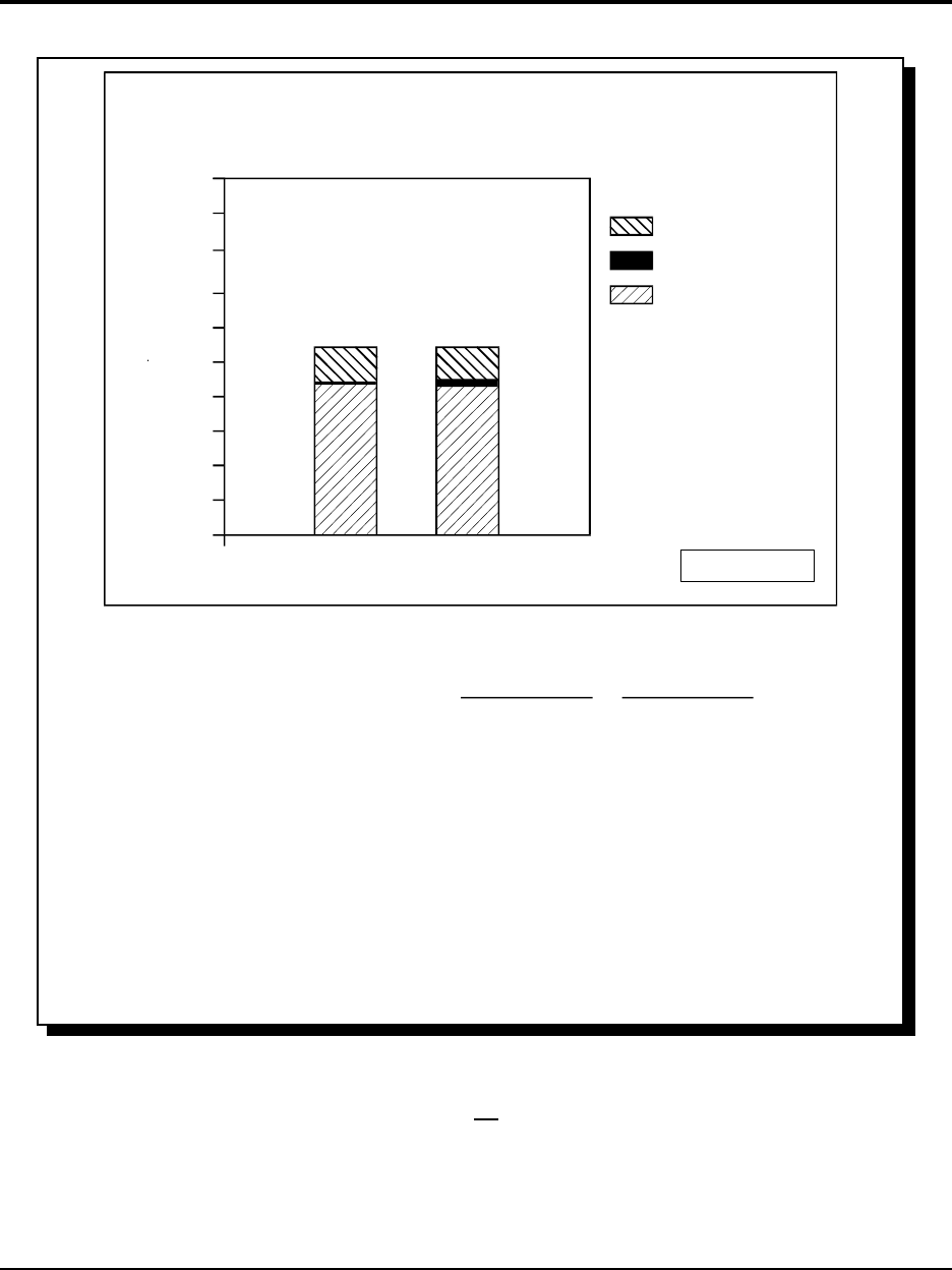
Figure 7-18 presents an historical perspective (1969 to 1994) for average speeds on freeways in

Harris County, Texas with a simple bar graph. The figure clearly illustrates that average speeds

dropped in the early 1980s, only to increase in the 1990s to original levels. A line graph could also

be used to illustrate time series speed or travel time trend.

Table 7-8 contains average speeds for freeways and arterial streets in Albuquerque, New Mexico.

The table contains the average speeds for the a.m. peak, p.m. peak, and both peak periods combined.

The total facility mileage is also included in the table to indicate the extent of each functional class.

Table 7-9 presents average speeds for several different functional classes in Harris County, Texas.

For each functional class, the table compares average speeds for different time periods and three

study years (e.g., 1988, 1991, 1994). Note that the table also includes the percentage change in

average speeds over the years illustrated. The inclusion of percent change in speed makes the time

series comparison easier to interpret.

Figure 7-19 shows several regional freeway speed trends using different types of graphical

presentations. Using bar graphs, the figure shows several dimension of congestion, including the

miles of congested freeway, the location of congestion, the congestion trend between 1969 and 1979,

and the congestion location trend between 1973 and 1979.

Figure 7-20 provides a summary of speed characteristics for all Class I arterial streets (as defined by

the 1994 Highway Capacity Manual) for data collected on streets in Houston, Texas. The speed

distributions presented in this figure are most appropriate for mobile source emissions modeling, in

which it is necessary to project the vehicle miles traveled (VMT) for various speed ranges. An

instrumented test vehicle is best suited for this application because the instrumentation is capable

of recording second-by-second changes in vehicle speed and acceleration.

Glendale 1979

Mesa 1979

Phoenix 1979

Scottsdale 1979

Tempe 1979

Glendale 1986

Mesa 1986

Phoenix 1986

Scottsdale 1986

Tempe 1986

0 10 20

Average Speed (km/h) 1 km = 0.6 mi

30 40 50 60 7

for Arterial Streets

Late Afternoon Period, 1979 and 1986

CHAPTER 7 - DATA REDUCTION, SUMMARY, AND PRESENTATION

7-36 Travel Time Data Collection Handbook

Source: adapted from reference (22)

Figure 7-17. Example of Functional Class Summary in Arizona Cities

47.1

43.3

41.6

38.3 38.3

41.1

45.6

46.3

49.4

1969 1973 1976 1979 1982

Year

1 km = 0.6 mi

AVERAGE PM SPEEDS ON HARRIS COUNTY

FREEWAYS IN PEAK DIRECTIONS (1969-1994

)

1985 1988 1991 1994

CHAPTER 7 - DATA REDUCTION, SUMMARY, AND PRESENTATION

Travel Time Data Collection Handbook 7-37

Average Speed (km/h)

Source: adapted from reference (23)

Figure 7-18. Example of Functional Class Summary in Harris County, Texas

CHAPTER 7 - DATA REDUCTION, SUMMARY, AND PRESENTATION

7-38 Travel Time Data Collection Handbook

Table 7-8. Example of Functional Class Summary for 1986 Albuquerque Travel Time Study

Functional Class

Average Speed, km/h

AM Peak PM Peak AM and PM Peak

All Streets Combined

Total Length 309.4 km 305.5 km 614.9 km

Mean Speed 43.6 km/h 41.9 km/h 42.7 km/h

Median Speed 41.7 km/h 40.7 km/h 41.4 km/h

Freeways

Total Length 58.0 km 55.9 km 113.9 km

Mean Speed 80.3 km/h 76.60 km/h 78.4 km/h

Median Speed 82.8 km/h 82.8 km/h 82.8 km/h

Arterials, Collectors, and

Ramps

Total Length 251.4 km 249.5 km 500.9 km

Mean Speed 40.6 km/h 38.7 km/h 39.7 km/h

Median Speed 40.8 km/h 39.7 km/h 40.6 km/h

Source: adapted from reference (24)

CHAPTER 7 - DATA REDUCTION, SUMMARY, AND PRESENTATION

Travel Time Data Collection Handbook 7-39

Table 7-9. Illustration of Functional Classification Summary for Harris County, Texas

Functional Roadway Extent (km) Average Speeds, km/h (for both directions of travel)

Class

AM Peak Off Peak PM Peak Total

1988 1991 1994 1988 1991 1994 •, 1988 1991 1994 •, 1988 1991 1994 •, 1988 1991 1994 •,

91-94 91-94 91-94 91-94

HOV Lanes - 82 101 - 87.1 80.7 -7 % - 94.5 86.1 - 9 % - 83.9 82.3 -2 % - 88.2 82.9 -6 %

Interstates 230 230 232 79.9 81.0 82.4 2 % 93.9 94.8 96.0 1 % 82.9 81.1 79.2 -2 % 85.2 85.2 85.3 0 %

Freeways 274 311 356 73.3 76.6 79.4 4 % 80.3 81.5 81.8 0 % 72.9 74.9 77.9 4 % 75.3 77.6 78.7 1 %

Principals 630 678 927 51.2 52.8 50.6 -4 % 53.3 53.9 53.6 -1 % 51.0 49.7 48.5 -3 % 51.8 52.0 50.9 -2 %

Arterials 765 407 164 44.9 46.9 44.0 -6 % 47.0 49.1 46.9 -5 % 44.3 43.8 44.9 3 % 45.4 46.5 45.2 -3 %

Totals 1,898 1,708 1,782 49.6 54.4 55.1 1 % 52.2 56.8 58.3 3 % 49.1 51.5 53.6 4 % 50.2 54.3 55.4 -3 %

Systemwide

Note: “•, 91-94" represents the percent change in average speeds between 1991 and 1994.

Source: adapted from reference (25)

CHAPTER 7 - DATA REDUCTION, SUMMARY, AND PRESENTATION

7-40 Travel Time Data Collection Handbook

Source: adapted from reference (16)

Figure 7-19. Example Summary of Congestion and Average Speed Trends

CHAPTER 7 - DATA REDUCTION, SUMMARY, AND PRESENTATION

7-42 Travel Time Data Collection Handbook

7.5.5 Other Summaries

There are several other travel time data summaries that do not fit neatly into any of the above

categories. Included in this group are activity center summaries, travel time contour maps, and

accessibility maps. Activity center summaries present trends or comparisons of travel time or

average speed between major activity centers in an urban area. Travel time contour maps use

isochronal lines (i.e., lines of equal time) to illustrate the distances that one can travel away from a

selected point (e.g., central business district (CBD) or major activity center) in given time intervals.

The isochronal lines are typically centered around a downtown or CBD area and are in ten-minute

increments. Accessibility maps show the accessibility (in terms of time increments) of land uses,

jobs, or services to transportation facilities.

In the past, the development of travel time contour and accessibility maps were considered time-

consuming and labor-intensive. The advent of geographic information systems (GIS) substantially

reduces the work and time required to prepare these types of graphical displays. Even if travel time

data are not collected with global positioning system (GPS) units, agencies may wish to consider

importing travel time data into a GIS platform for the ease of future analyses.

Table 7-10 shows an example of an activity center travel time matrix for Harris County, Texas (this

table has been shortened from the original travel time matrix). The table shows travel times between

major activity centers for three different time periods during the day: off peak, a.m. peak, and p.m.

peak. The travel times shown are for the most direct route and may include portions of several

different arterial streets and/or freeways.

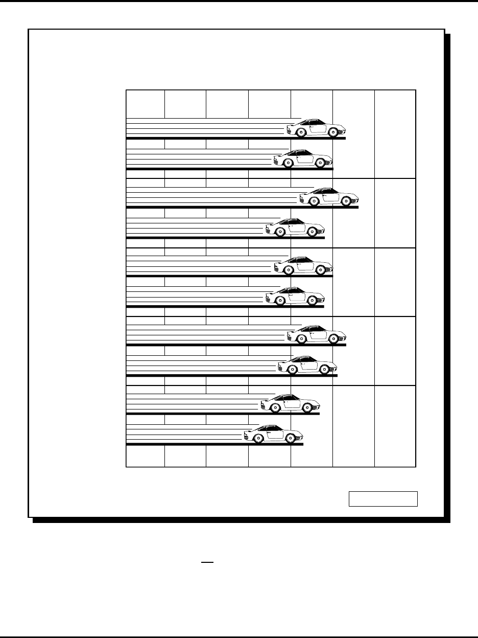
Figure 7-21 illustrates average speeds between major activity centers and two airports in the

Philadelphia area. The average speeds are compared for two years, 1971 and 1983. As with the

activity center matrix in Table 7-10, the average speeds shown in Figure 7-21 presumably contain

portions of trips on arterial streets and/or freeways.

Figure 7-22 shows an example of a travel time contour map that compares average travel times

between 1980 and 1991. The decreases in mobility can be seen from the shaded areas. Travel time

contour maps can be used to show many regional trends relating to mobility:

• Trends over time (e.g., historical comparisons every five years);

• Differences between peak and off-peak traffic conditions;

• Reliability of travel times;

• Comparison of transportation alternatives; and,

• Trends before and after regional transportation improvements.

Figure 7-23 shows an example of an accessibility map for a proposed transportation improvement

(i.e., Inter-County Connector) in Montgomery County, Maryland. In this example, the figures show

CHAPTER 7 - DATA REDUCTION, SUMMARY, AND PRESENTATION

Travel Time Data Collection Handbook 7-43

the accessibility to jobs within a 45-minute commute, and the additional accessibility to jobs created

by the transportation improvement.

Table 7-10. Example of Activity Center Travel Time Matrix

From Time

Period

Travel Time (minutes) to

CBD MED ASTR HOBBY INTRC CLR LK SGLD

CTR

CBD Off Peak - 11 11 17 25 26 27

Main @ McKinney AM Peak - 9 13 16 25 27 27

(CBD) PM Peak - 10 14 24 28 38 39

Medical Center Off Peak 11 - 6 19 31 29 24

Main @ University AM Peak 8 - 6 19 33 29 24

(MED CTR) PM Peak 10 - 8 28 39 41 34

Astrodome Off Peak 11 6 - 13 30 22 20

Kirby @ IH 610 AM Peak 13 6 - 13 31 22 22

(ASTR) PM Peak 12 7 - 19 36 33 27

Hobby Airport Off Peak 17 19 13 - 33 14 32

Airport Entrance AM Peak 19 21 14 - 36 14 36

(HOBBY) PM Peak 19 25 17 - 40 16 45

Intercontinental Airport Off Peak 25 34 30 34 - 43 44

Terminal B AM Peak 27 37 36 35 - 45 47

(INTRC) PM Peak 25 35 31 41 - 52 48

Clear Lake City Off Peak 26 28 22 15 43 - 41

Bay Area Blvd@IH 45S AM Peak 33 36 29 18 51 - 50

(CLR LK) PM Peak 25 31 24 15 46 - 51

Sugar Land Off Peak 27 26 22 34 45 43 -

SH 6 @ US 59S AM Peak 37 34 28 41 48 50 -

(SGLD) PM Peak 26 24 21 40 48 53 -

Source: Houston-Galveston Regional Transportation Study, 1991.

Philadelphia Trenton Wilmington King of

Cherry

Langhorne Bordentown Trenton Princeton Bordentown Langhorne

1983

1971

LEGEND

PHILADELPHIA INTERNATIONAL AIRPORT MERCER COUNTY AIRPORT

Philadelphia International and Mercer County Airports

Avg. Speed (km/h)

CHAPTER 7 - DATA REDUCTION, SUMMARY, AND PRESENTATION

7-44 Travel Time Data Collection Handbook

Source: adapted from reference (27)

Figure 7-21. Example of Activity Center Average Speed Comparison in Philadelphia, Pennsylvania

0 3 6 km

Improved Mobility

(1981 to 1990)

Decreased Mobility

(1981 to 1990)

- Dayton CBD

CHAPTER 7 - DATA REDUCTION, SUMMARY, AND PRESENTATION

Travel Time Data Collection Handbook 7-45

Source: adapted from reference (28).

Figure 7-22. Example of a Travel Time Contour Map

Gaithersburg

Rock Creek

Olney

Fairland

Shady Grove

Beltsville

Rockville

Muirkirk

Aspen Hill

Laurel

Kensington

Freeways

0-25,000

Jobs Access. by Transit

LEGEND

MARC Brunswick

25,001-100,000

Metro Red Line 100,001-250,000

Metro Green Line 250,000+

I-495

White Oak

I-270

Source: Metropolitan Washington Council of Governments, 1996.

Figure 7-23. Example of an Accessibility Map for Montgomery County, Maryland

7-46 Travel Time Data Collection Handbook

CHAPTER 7 - DATA REDUCTION, SUMMARY, AND PRESENTATION

Travel Time Data Collection Handbook 7-47

Other good examples of travel time or speed summaries can be found on the World Wide Web.

Tens of thousands of daily commuters rely on these web page summaries for real-time information

on travel times and speeds. Because of the dynamic nature of these pages, several examples are

referenced below for the reader to explore. The following are examples of web pages that provide

real-time travel time or speed information:

• Atlanta, Georgia: http://www.georgia-traveler.com/traffic/rtmap.htm

• Gary-Chicago-Milwaukee: http://www.ai.eecs.uic.edu/GCM/GCM.html

• Houston, Texas: http://traffic.tamu.edu/traffic.html

• Houston, Texas: http://www.accutraffic.com/accuinfo/cities/houston.tx/

• Long Island, New York: http://metrocommute.com:81/LI/#heading

• Los Angeles, California: http://www.scubed.com/caltrans/la/la_big_map.shtml

• Minneapolis-St. Paul, Minnesota: http://www.traffic.connects.com/

• Orange County, Ca: http://www.maxwell.com/yahootraffic/OC/OC_W/map.html

• Phoenix, Arizona: http://www.azfms.com/Travel/freeway.html

• San Diego, California: http://www.scubed.com/caltrans/sd/big_map.shtml

CHAPTER 7 - DATA REDUCTION, SUMMARY, AND PRESENTATION

7-48 Travel Time Data Collection Handbook

1. Quiroga, C.A. “An Integrated GPS-GIS Methodology for Performing Travel Time Studies.”

Louisiana State University Ph.D. Dissertation, Baton Rouge, Louisiana, 171 p., 1997.

2. Quiroga, C.A. and D. Bullock. “Development of CMS Monitoring Procedures.” Draft Final

Report, Louisiana Transportation Research Center, Baton Rouge, Louisiana, April 1998.

3. Eisele, W.L., S.M. Turner and R. J. Benz. Using Acceleration Characteristics in Air Quality

and Energy Consumption Analyses. Report No. SWUTC/96/465100-1, Southwest Region

University Transportation Center, Texas Transportation Institute, August 1996.

4. Lomax, T., S. Turner, G. Shunk, H.S. Levinson, R.H. Pratt, P.N. Bay, and G.B. Douglas.

Quantifying Congestion: User’s Guide. NCHRP Report 398: Volume II, TRB, Washington,

DC, November 1997.

5. Liu, T.K. and M. Haines. Travel Time Data Collection Field Tests - Lessons Learned.

Report FHWA-PL-96-010. U.S. Department of Transportation, Federal Highway

Administration, Washington, DC, January 1996.

6. Quiroga, C.A. and D. Bullock, “Measuring Delay at Signalized Intersections Using GPS.”

Draft paper submitted to the ASCE Journal of Transportation Engineering, 1998.

7. Cullison, J., R. Benz, S. Turner, and C. Weatherby. Dallas Area Rapid Transit (DART)

Light Rail Transit Starter System Parallel Facility Travel Time Study: Before Conditions.

North Central Texas Council of Governments, Texas Transportation Institute, Texas A&M

University System, College Station, Texas, August 1996.

8. Robertson, H.D., ed. Manual of Transportation Engineering Studies. Institute of

Transportation Engineers, Washington, D.C., 1994.

9. Hampton Roads Planning District Commission. Southeastern Virginia Regional Travel Time

1990: Volume 2. Chesapeake, Virginia, January 1991.

10. Indian Nations Council of Governments. Travel Time and Delay Study. Tulsa, Oklahoma,

April 1990.

11. Hampton Roads Planning District Commission. Southeastern Virginia Regional Travel Time

1990: Volume 1. Chesapeake, Virginia, January 1991.

12. Benz, R.J., D.E. Morris and E.C. Crowe. Houston-Galveston Regional Transportation

Study: 1994 Travel Time and Speed Survey, Volume I - Executive Summary. Texas

Department of Transportation, Texas Transportation Institute, Texas A&M University,

7.6 References for Chapter 7

CHAPTER 7 - DATA REDUCTION, SUMMARY, AND PRESENTATION

Travel Time Data Collection Handbook 7-49

College Station, Texas, May 1995.

13. Bullock, D., C. Quiroga, and N. Kamath. “Data Collection and Reporting for Congestion

Management Systems.” In National Traffic Data Acquisition Conference (NATDAC ‘96)

Proceedings, Volume I. Report No. NM-NATDAC-96, Alliance for Transportation

Research, Albuquerque, New Mexico, May 1996, pp. 136-146.

14. Bullock, D. and C.A. Quiroga. Development of a Congestion Management System Using

GPS Technology. Final Report - Volume I, Louisiana Transportation Research Center, Baton

Rouge, Louisiana, April 1997.

15. Northeast Ohio Areawide Coordinating Agency. I-77 Traffic Report. April 1990.

16. “1979 Travel Time and Speed Survey.” Houston-Galveston Regional Transportation Study,

1980.

17. Turner, S.M. Advanced Techniques for Travel Time Data Collection. In Transportation

Research Record 1551. TRB, National Research Council, Washington, DC, 1996.

18. TMATS Travel Time Study. Tulsa Metropolitan Area Planning Commission, Tulsa,

Oklahoma, September 1979.

19. Turner, Shawn M., Using ITS Data for Transportation System Performance Measurement.

In Traffic Congestion and Traffic Safety in the 21 Century: Challenges, Innovations, and

Opportunities. American Society of Civil Engineers, New York, New York, June 1997.

20. Ogden, M.A. and D.E. Morris. Houston-Galveston Regional Transportation Study: 1991

Travel Time and Speed Survey, Volume I - Executive Summary. Texas Department of

Transportation, Texas Transportation Institute, Texas A&M University, College Station,

Texas, March 1992.

21. Travel Time Study, Report II: Speed Characteristics. Chicago Area Transportation Study,

Chicago, Illinois, March 1982.

22. Parsons Brinckerhoff. 1986 Phoenix Urbanized Area Travel Speed Study: Final Report.

Arizona Department of Transportation, Transportation Planning Division, 1986.

23. “H-GRTS Newsletter.” Vol. 24, No. 2. Texas Department of Transportation, Houston-

Galveston Regional Transportation Study, Fall 1995.

24. 1986 Travel Time Study for the Albuquerque Urbanized Area. Report TR-100, Middle Rio

Grande Council of Governments, Albuquerque, New Mexico, June 1987.

CHAPTER 7 - DATA REDUCTION, SUMMARY, AND PRESENTATION

7-50 Travel Time Data Collection Handbook

25. Benz, R.J., D.E. Morris and E.C. Crowe. Houston-Galveston Regional Transportation

Study: 1994 Travel Time and Speed Survey, Volume I - Executive Summary. Texas

Department of Transportation, Texas Transportation Institute, Texas A&M University,

College Station, Texas, May 1995.

26. Eisele, W.L., S.M. Turner, and R.J. Benz. Using Acceleration Characteristics in Air Quality

and Energy Consumption Analyses. Report No. SWUTC/96/465100-1. Southwest Region

University Transportation Research Center, Texas Transportation Institute, College Station,

Texas, August 1996.

27. Highway Travel Time Between Major Regional Activity Centers and the Philadelphia

International and Mercer County Airports. Delaware Valley Regional Planning

Commission, February 1984.

28. “Transportation Communications: 1990 Travel Time Report for the Dayton Urbanized

Area.” Technical Report. Miami Valley Regional Planning Commission, Dayton, Ohio,

August 1990.