A Thesis By JUAN RUFINO MORGA REYES, 51198208 Master of

A Thesis By

JUAN RUFINO MORGA REYES, 51198208

Master of Public Policy, International Program (MPP/IP)

(Economic Policy, Finance, and Development)

PROFESSOR KONSTANTIN KUCHERYAVYY (PH.D.)

Academic Supervisor

GRADUATE SCHOOL OF PUBLIC POLICY

THE UNIVERSITY OF TOKYO

TOKYO, JAPAN

JUNE 2021

DECLARATION

I hereby declare that this thesis is my original work, and I have written it in its entirety.

I have duly acknowledged all the sources of information that have been used in this research.

In addition, this study has not been submitted for any degree or university previously.

(Sgd.)

JUAN RUFINO M. REYES, 51198208

Master of Public Policy, International Program (MPP/IP)

Graduate School of Public Policy

The University of Tokyo

ACKNOWLEDGEMENT

First of all, I would like to express my deepest gratitude to my academic supervisor,

Professor Konstantin Kucheryavyy (Ph.D.), for imparting his knowledge on data science and

providing technical assistance for this research. I appreciate the effort and encouragement you

conveyed during the entire thesis writing process. Thank you for the patience you have shown

and for the remarkable recommendations for this thesis.

I also would like to thank the (1) Joint Japan/World Bank Graduate Scholarship

Program (JJ/WBGSP) for giving me the opportunity and support to study at the most

prestigious university in Japan, The University of Tokyo (UTokyo); and

(2) Bangko Sentral ng Pilipinas (BSP) for allowing me to pursue a degree in the field of

public policy (i.e., economic policy, finance, and development) to become a better central banker

that could contribute to the development of monetary policy in the Philippines.

To the significant contributors of data in this thesis: Mr. Justin Parco of

Investor Relations Office (IRO), colleagues at the Department of Economic Statistics (DES),

and International Operations Department (IOD) of the BSP, I appreciate your generosity in

providing relevant statistics despite your busy schedules. Thank you for your

kind understanding.

Lastly, I am particularly thankful to Ms. Mia Agcaoili, my parents

(Engr. Rico and Marylen Reyes), and my siblings (Ms. Michelle and Ana Reyes) for

their unending love and support. I am forever grateful for your encouragement that

I can produce a study that is timely and relevant. Thank you for believing that this

thesis could be one of the best!

TABLE OF CONTENTS

DECLARATION

ACKNOWLEDGEMENT

TABLE OF CONTENTS

ABSTRACT

ACRONYMS

LIST OF TABLES

LIST OF FIGURES

PART ONE

RESEARCH FRAMEWORK:

BACKGROUND, THEORY, AND METHODOLOGY OF THE STUDY

CHAPTER I: INTRODUCTION

1.1. Background of the Study 2

1.1.1. Economic Nowcasting, Big Data, and Machine Learning 3

1.1.2. The Philippines and Domestic Liquidity 6

1.2. Statement of the Problem 8

1.3. Research Objectives 10

1.4. Significance of the Study 10

1.5. Scope and Limitations 11

1.6. Definition of Terms 12

CHAPTER II: REVIEW OF RELATED LITERATURE

2.1. Primer 14

2.2. Regularization Methods 15

2.3. Tree-Based Methods 19

2.4. The Utilization of Two (2) Machine Learning Methods 23

CHAPTER III: RESEARCH METHODOLOGY

3.1. Primer 26

3.2. Models 26

3.2.1. Benchmark Models 27

3.2.1.1. Autoregressive Models 27

3.2.1.1.1. Autoregressive Integrated Moving Average 27

3.2.1.1.2. Random Walk 28

3.2.1.2. Vector Autoregression 28

3.2.1.3. Dynamic Factor Model 29

3.2.2. Machine Learning Models 30

3.2.2.1. Regularization Methods 30

3.2.2.1.1. Ridge Regression 30

3.2.2.1.2. Least Absolute Shrinkage and Selection Operator 31

3.2.2.1.3. Elastic Net 32

3.2.2.2. Tree-Based Methods 32

3.2.2.2.1. Decision Tree 33

3.2.2.2.2. Random Forest 34

3.2.2.2.3. Gradient Boosted Trees 34

3.3. Nowcast Evaluation Methodology 35

3.4. Research Tool 36

PART TWO

RESEARCH ANALYSIS:

DATA AND EMPIRICAL RESULTS

CHAPTER IV: DATA AND DIAGNOSTICS

4.1. Primer 38

4.2. Data 38

4.2.1. Target Variable 38

4.2.2. Input Variables 38

4.2.2.1. Monetary Indicators 39

4.2.2.2. Financial Indicators 40

4.2.2.3. External Indicators 41

4.2.2.4. Lagged Values of Domestic Liquidity 41

4.3. Averaging and Interpolation 41

4.3.1. Averaging of High Frequency Variables 42

4.3.2. Interpolation of Low Frequency Variables 42

4.4. Diagnostics and Feature Engineering 43

4.4.1. Seasonal Adjustment 43

4.4.2. Logarithmic Transformation 43

4.4.3. Stationarity 43

CHAPTER V: EMPIRICAL RESULTS AND ANALYSIS

5.1. Primer 46

5.2. Calibration and Nowcast Results 46

5.2.1. One-Step-Ahead (Out-of-Sample) via Expanding Window 46

5.2.2. Autoregressive Models 47

5.2.2.1. Model Calibration 47

5.2.2.2. Nowcast Results 49

5.2.3. Dynamic Factor Model 51

5.2.3.1. Model Calibration 51

5.2.3.2. Nowcast Results 52

5.2.4. Machine Learning Models 54

5.2.4.1. Regularization Methods 54

5.2.4.1.1. Model Calibration 54

5.2.4.1.2. Nowcast Results 55

5.2.4.2. Tree-Based Methods 57

5.2.4.2.1. Model Calibration 57

5.2.4.2.2. Nowcast Results 59

5.3. Further Analysis 61

5.3.1. Variable Importance 61

5.3.1.1. LASSO and ENET 61

5.3.1.2. Random Forest and Gradient Boosted Trees 62

PART THREE

FINAL CHAPTERS

CHAPTER VI: CONCLUSION

6.1. Summary and Conclusion 65

CHAPTER VII: RECOMMENDATION

7.1. Potential Actions 69

7.2. Suggestions for Future Research 70

BIBLIOGRAPHY

ANNEXES

Annex A R Studio Packages

Annex B Unit Root Tests for Input Variables

Annex C Optimal Shrinkage Penalty via Ridge Regression

Annex D Optimal Shrinkage Penalty via LASSO

Annex E Optimal Shrinkage Penalty via ENET

Annex F OOB Error of Training Datasets via Random Forest

Annex G Optimal Number of Trees via Gradient Boosted Trees

Annex H Variable Coefficients via LASSO: January to December 2020

Annex I Variable Coefficients via ENET: January to December 2020

ABSTRACT

1

,

2

Domestic liquidity (also known as broad money) is defined as the sum of all

liquid financial instruments held by money-holding sectors that are used as a

medium of exchange in an economy (IMF, 2016). The changes in the overall growth of this

monetary indicator are among the most important dynamics that numerous central banks are

closely monitoring. This is because of its property of being an essential element to the

overall transmission mechanism of monetary policy, particularly the impact of

money supply expansion or contraction on aggregate demand, interest rates, inflation, and

overall economic growth (Mankiw, n.d.).

In the Philippines, data on domestic liquidity is used as a primary component

to formulate monetary policy and utilized as a leading indicator to observe

price and financial stability. However, similar to the concerns regarding the delayed publication

of data or statistical indicators generated by most government offices, data on domestic liquidity

in the said country also suffers from series of lags and revisions. Due to this predicament,

policymakers in the Central Bank of the Philippines or Bangko Sentral ng Pilipinas (BSP)

typically formulate monetary policies and address different economic phenomena (e.g., inflation,

business cycle) using its outdated or lagged values.

The concept of short-

methodologies utilized by numerous institutions (e.g., International Financial Institutions (IFIs),

central banks) to address the aforementioned issues in data publication. This approach,

at present, also became prevalent because of the emergence of big data and machine learning

which augment its overall process (Hassani and Silva, 2015; Richardson et al., 2018).

1

juanrufin[email protected]; juanrufinom[email protected]tokyo.ac.jp

2

The results expressed herein do not represent the views nor opinions of GraSPP, UTokyo, as well as the BSP. Errors and omissions

are sole responsibility of the author.

That being said, this study aims to utilize machine learning algorithms to provide an

optimal model to nowcast the growth of domestic liquidity in the Philippines.

In particular, the following steps are performed to support this objective:

(1) perform one-step-ahead (out-of-sample) nowcasts through regularization

(i.e., Ridge Regression, Least Absolute Shrinkage and Selection Operator (LASSO),

Elastic Net (ENET)) and tree-based methods (i.e., Random Forest (RF),

Gradient Boosted Trees (GBT)); (2) recognize and compare the accuracy of each algorithm

vis-à-vis traditional time series models used in economic forecasting, such as

Autoregressive (AR) Models and Dynamic Factor Model (DFM); and (3) systematically identify

important high-frequency variables (i.e., monetary, financial, external sector) that could

accurately nowcast domestic liquidity in the Philippines.

Based on the conducted recursive nowcasts from January to December 2020,

it was found that machine learning algorithms provide more accurate estimates than the

traditional time series models utilized in this study. This is due from the consistent

monthly estimates with low forecast errors (i.e., Root Mean Square Error, Mean Absolute Error)

that the machine learning algorithms registered. The said quantitative models also registered

precise nowcasts on the months where domestic liquidity growth suddenly expand

(e.g., increased borrowings and deposits of National Government to BSP) due to the impact of

Coronavirus Disease 2019 (COVID-19) in the Philippines. Further, the results indicate that

regularization methods are the most optimal machine learning algorithms to nowcast the

aforementioned monetary indicator.

This study also concludes that using regularization methods, such as

LASSO and ENET, as well as tree-based methods, such as RF and GBT, are useful in

filtering out or identifying important indicators that stipulate parsimonious nowcasting models

with precise results.

Keywords: Domestic Liquidity, Machine Learning, Nowcasting, Philippines

ACRONYMS

ACF Autocorrelation Function

ADB Asian Development Bank

ADF Augmented Dickey-Fuller Test

AIC Akaike Information Criterion

ARC Advance Release Calendar

ARIMA Autoregressive Integrated Moving Average

AT Adaptive Trees

BOP Balance of Payments

BSP Bangko Sentral ng Pilipinas

BVAR Bayesian Vector Autoregression

CBS Central Bank Survey

CDS Credit Default Swap

COVID-19 Coronavirus Disease 2019

CPI Consumer Price Index

DCS Depository Corporations Survey

DES Department of Economic Statistics

DFM Dynamic Factor Model

ENET Elastic Net

EWS Early Warning System

FOF Flow of Funds

FOREX Foreign Exchange Rate

FPI Foreign Portfolio Investment

GBT Gradient Boosted Trees

GDP Gross Domestic Product

HQ Hannan-Quinn Information Criterion

IFI International Financial Institutions

IMF International Monetary Fund

IOD International Operations Department

LASSO Least Absolute Shrinkage and Selection Operator

LIBOR London Interbank Offered Rates

LSM Large-Scale Manufacturing

M1 Monetary Base

M2 M1 and Savings/Time Deposits

M3 Domestic Liquidity

MAE Mean Absolute Error

MAFE Mean Absolute Forecast Error

MFSM Monetary and Financial Statistics Manual

MSFE Mean Squared Forecast Error

NG National Government

NGA National Government Agencies

ODC Other Depository Corporations

OLS Ordinary Least Squares

OOB Out-of-Bag Error

PACF Partial Autocorrelation Function

PBS Philippine Banking System

PHIREF Philippine Interbank Reference Rate

PP Philipps-Perron Test

RF Random Forest

RMSE Root Mean Square Error

RSS Residual Sum of Squares

RW Random Walk

SARIMA Seasonal Autoregressive Integrated Moving Average

SIBOR Singapore Interbank Offered Rates

VAR Vector Autoregression

WB World Bank Group

WEO World Economic Outlook

WMOR Weighted Monetary Operations Rate

YOY Year-on-Year

LIST OF TABLES

Table 1.1 Depository Corporations Survey (Date Accessed: 10 April 2021)

Table 4.1 Summary Statistics of Domestic Liquidity in the Philippines

Table 4.2 List of Data

Table 4.3 Unit Root Tests for Domestic Liquidity in the Philippines

Table 5.1 RMSE of Autoregressive Models

Table 5.2 MAE of Autoregressive Models

Table 5.3 RMSE of DFM

Table 5.4 MAE of DFM

Table 5.5 RMSE of Ridge Regression, LASSO, and ENET

Table 5.6 MAE of Ridge Regression, LASSO, and ENET

Table 5.7 RMSE of RF and GBT

Table 5.8 MAE of RF and GBT

Table 5.9 Variable Coefficients via LASSO and ENET (Jan.-Feb. 2020)

Table 6.1 RMSE of Benchmark and Machine Learning Models (Summary)

Table 6.2 MAE of Benchmark and Machine Learning Models (Summary)

LIST OF FIGURES

Figure 3.1 Decision Tree Growing Process

Figure 3.2 Expanding Window Process

Figure 4.1(a) Domestic Liquidity in the Philippines (Levels, in Million PHP)

Figure 4.1(b) Domestic Liquidity in the Philippines (Growth Rate, in Percent)

Figure 4.2(b) Domestic Liquidity in the Philippines (Growth Rate, in First Diff.)

Figure 4.3 Research Workflow Diagram

Figure 5.1(a) ACF of M3 (Seasonally Adjusted)

Figure 5.1(b) PACF of M3 (Seasonally Adjusted)

Figure 5.2 Residual Plot for ARIMA (4,1,1)

Figure 5.3 Autoregressive Model Nowcasts vs. Actual M3 Growth (in Percent)

Figure 5.4 Eigenvalues of Input Variables via Factor Analysis

Figure 5.5 DFM Nowcasts vs. Actual M3 Growth (in Percent Diff.)

Figure 5.6(a) Overall RMSE of Autoregressive Models and DFM

Figure 5.6(b) Overall MAE of Autoregressive Models and DFM

Figure 5.7 Optimal Shrinkage Penalty via Ridge Regression

Figure 5.8 Regularization Nowcasts vs. Actual M3 Growth (in Percent Diff.)

Figure 5.9(a) Overall RMSE of Benchmark Models and Regularization Methods

Figure 5.9(b) Overall MAE of Benchmark Models and Regularization Methods

Figure 5.10 OOB Error of Training Datasets via Random Forest

Figure 5.11 Optimal Number of Trees via Gradient Boosted Trees

Figure 5.12 Tree-Based Method Nowcasts vs. Actual M3 Growth (in Percent Diff.)

Figure 5.13(a) Overall RMSE of Benchmark Models and Tree-Based Methods

Figure 5.13(b) Overall MAE of Benchmark Models and Tree-Based Methods

Figure 5.14 Node Impurity via Random Forest

Figure 5.15 Variable Importance Plot via Gradient Boosted Trees

Figure 6.1 Overall Forecast Errors of Benchmark and Machine Learning Models

- this page left intentionally blank -

1

CHAPTER I: INTRODUCTION

CHAPTER II: REVIEW OF RELATED LITERATURE

CHAPTER III: RESEARCH METHODOLOGY

2

Chapter I:

INTRODUCTION

1.1. Background of the Study

Understanding the current condition of their respective economy is essential

for every policymaker around the world. Therefore, timely announcements of various

macroeconomic indicators (e.g., monetary, national accounts) are important for them to be able

to monitor the current growth of different economic sectors comprehensively (e.g., households,

other depository corporations) as well as to formulate and implement strong policy

(e.g., fiscal, monetary) responses. Proponents of high-quality public data management,

such as the International Monetary Fund (IMF), argued that having reliable and sensible

datasets are essential to depict the overall condition of an economy and to strictly monitor

if any negative externalities could cause a financial crisis. Hence, numerous government offices

(e.g., central banks, finance ministries) are transforming their approach to ensure that

macroeconomic indicators are published in a timely and consistent manner

(Carriere-Swallow and Haskar, 2019).

Adopting these data management principles, however, cannot be easily implemented in

every country. This is because of the tedious and complicated processes that each

government office must perform to produce numerous macroeconomic indicators promptly.

The proper classification of accounts, changes in the overall compilation framework, and

inevitable delays in receiving input documents are among the few reasons that coerced the

delay in publishing data at the national level (Dafnai and Sidi, 2010;

Chikamatsu et al., 2018). Recent studies discussed that national government agencies (NGAs)

and central banks from different advanced (e.g., United States (US), Japan, New Zealand) and

emerging economies (e.g., Israel, Lebanon) had encountered this difficulty

(Dafnai and Sidi, 2010; Bragoli and Modugno, 2016; Chikamatsu et al., 2018;

Richardson et al., 2018). Due to this predicament, policymakers from these countries are forced

3

to formulate policies and address several economic phenomena (e.g., inflation, business cycle)

using non-related, outdated, or lagged datasets (Richardson et al., 2018).

To systematically address this concern, short-

of the recently introduced methodologies by different International Financial Institutions (IFIs),

NGAs, and central banks. This is because of its strong capacity to observe the overall state of

an economy or any target variable of interest using conventional and unconventional data

as well as high-frequency indicators that are usually published at an earlier date (Tiffin, 2016).

Due to the difficulty in producing official macroeconomic indicators on a real-time basis,

nowcasting has been the alternative approach used by said institutions to systemically

estimate the official figure of a specific set of information before it becomes available

Asian Development Bank (ADB) are

among the IFIs that conducted comprehensive studies regarding the use of nowcasting in

different fields of study (e.g., economics, finance). Meanwhile, central banks of Indonesia, Israel,

Japan, and New Zealand are among the well-known institutions that attempted to use the said

concept to estimate the short-run growth of their respective Gross Domestic Product (GDP) and

Consumer Price Index (CPI).

3

1.1.1. Economic Nowcasting, Big Data, and Machine Learning

For the past years, predicting the overall growth of an economy, the progress of a

particular economic sector, and the transmission mechanism of policies are commonly performed

through economic forecasting using time series analysis. This approach has been the traditional

forecasting methodology under the field of economics (or econometrics) because numerous studies

have already established its capacity to provide a clear and substantial outlook of different

macro and socioeconomic indicators, such as GDP, CPI, and poverty incidence, among others.

Aside from this, the said approach is frequently used by various well-known institutions to

estimate the dynamic effects of policy implementation on the overall economic growth of their

3

See Dafnai and Sidi (2010), Chikamatsu et al. (2018), Richardson et al. (2018), and Tamara et al. (2020).

4

respective country. Among the numerous time series models used in economic forecasting are

Autoregressive (AR), Vector Autoregressive (VAR), and Dynamic Factor Models (DFM).

4

However, in most cases, time series models used in economic forecasting are

highly dependent on the timeliness of data or information. Therefore, any delay in the

publication process of the explanatory variable(s) included in a particular forecasting model

could hamper the attempt to predict the future condition of the target output.

For instance, to predict the GDP for Q2:2020 using a simple AR(1) model, its figure as of

end-Q1:2020 is strongly needed.

5

However, in a typical situation, the publication of GDP for

Q1:2020 is not released exactly at the end of said period. The latest figures are typically posted

one (1) or two (2) months after the reference date (e.g., GDP for Q2:2020 is published in

August 2020, rather than end-June 2020).

6

Therefore, an individual or institution that aims to

forecast the economic growth for Q2:2020 using an AR(1) model should wait until the GDP as

of end-Q1:2020 is published.

This concern was one of the main reasons that pushed numerous individuals and

institutions to adopt the concept of nowcasting in the field of economics. This is because of its

capacity to exploit multiple real-time data or information (e.g., daily financial data,

survey results) to accurately estimate the present, near future, and recent past of a particular

macro or socioeconomic variable l., 2013, Chikamatsu et al., 2018;

Richardson et al., 2018). For example, to predict the current state of an economy,

high-frequency data or information (e.g., trade balances, financial data) that signals the current

GDP can be utilized before associated official GDP figures are published (Tiffin, 2016).

Moreover, since most conventional macroeconomic indicators are published with lags and

frequent revisions, nowcasting became an essential tool for policymakers to minimize the

usual approach of addressing different economic phenomena using non-related, outdated, or

lagged data (Richardson et al., 2018).

4

See Hang (2010), Ikoku (2014), Doguwa and Alade (2015), and Rajapov and Axmadjonov (2018).

5

Autoregressive Model of Order 1 or AR(1) model is defined as .

6

Depending on the statistical calendar (or advance release calendar) of a specific country.

5

The stu

In particular, the authors mentioned that:

Nowcasting is relevant in economics because key statistics on the

present state of the economy are available with a

significant delay. This is particularly true for those collected

on a quarterly basis, with GDP being a prominent example.

For instance, the first official estimate of GDP in the United States

or in the United Kingdom is published approximately

one month after the end of the reference quarter.

In the Euro area, the corresponding publication lag is two (2) to

three (3) weeks longer. Nowcasting can also be meaningfully applied

to other target variables revealing particular aspects of the state of

the economy and thereby followed closely by markets (p. 2).

Aside from the institutional concern, another factor that contributed to the emergence

of nowcasting is the recent trend in the use of big data and machine learning.

7

,

8

The rise of these concepts improved the overall effectiveness of nowcasting in the

field of economics because of two (2) particular reasons. The first reason is that the former has

a strong potential to provide complementary information with respect to the macroeconomic

data that government offices usually published (Baldacci et al., 2016). Meanwhile, the latter has

the capacity to utilize the immense amount of data or information that the former concept

provided (Hassani and Silva, 2015; Richardson et al., 2018). In addition to economics, conducting

nowcasting through big data and machine learning is also performed by different individuals and

institutions in the fields of energy, medicine, and population dynamics. This is because the said

approach was found to be an essential tool to have an accurate short-term forecast,

7

Big data is defined as large datasets that can be examined computationally to observe different patterns, trends, among others .

8

Machine learning refers to the use of computer system, algorithms, and/or statistical models to analyze and draw conclusions from

patterns in data.

6

which further improves the decision-making as well as policy formulation and implementation of

individuals or institutions under these fields (Hassani and Silva, 2015).

1.1.2. The Philippines and Domestic Liquidity

Domestic liquidity is defined as the total amount of money available in an economy that

is usually determined by a central bank and banking system (Mankiw, n.d. p. 623).

9

In particular, as stated under the Monetary and Financial Statistics Manual (MSFM) of the

IMF, the said monetary indicator is the sum of all liquid financial instruments held by

money-holding sectors, such as Other Depository Corporations (ODCs). It can be categorized as

a particular commodity that is widely accepted as (1) medium of exchange and

(2) close substitute for the medium of exchange that has a reliable store value

(IMF, 2016 p. 180).

10

,

11

The change in the overall growth of this monetary indicator is one of the most important

dynamics that most central banks are closely monitoring. Mainly because it is an

essential element to the transmission mechanism of monetary policy, particularly the

impact of money supply expansion or contraction on aggregate demand, interest rates,

inflation, and overall economic growth. For this reason, policymakers in different central banks

passionately observe its current and future development to formulate an effective and timely

monetary policy response, especially when there are seen predicaments that require them to

adjust policy rates and the overall monetary base (Mankiw, n.d.).

Similar to its role in every economy across regions, domestic liquidity likewise holds a

critical function in the economy of the Philippines. Both the level and growth of said

monetary indicator are usually being monitored by its central bank otherwise known as the

9

The words domestic liquidity, broad money, money supply, money demand, and M3 are interchangeably used in this paper.

10

The MFSM is the official guideline of IMF member countries in compiling and presenting monetary statistics.

11

ODCs refers to financial corporations (other than the central bank) that incur liabilities included in domestic liquidity

(IMF, 2016 p. 405).

7

Bangko Sentral ng Pilipinas (BSP) because it is also primarily used as the measurement of

liquidity in the country, input for early warning system (EWS) models on the macroeconomy,

and principal data to formulate and implement monetary policy, among others.

12

Money supply in the Philippines has a similar structure with most countries with

fractional-reserve banking systems (e.g., US, Japan).

13

Mainly because bank reserves,

currency deposits (or monetary base), and other liquid financial instruments are likewise its

main components. In particular, based on the Depository Corporations Survey (DCS) conducted

by the BSP, broad money in the said country is mainly composed of currency in circulation and

transferable deposits (M1), other deposits such as savings and time deposits (M2), and

deposit substitutes such as debt instruments (BSP, 2018).

14

On a monthly basis, the BSP announces the current level and growth of broad money in

the Philippines. However, for the said monetary indicator to be released in a timely manner,

the said institution needs to strictly ensure that the monthly submission of bank reports

(e.g., balance sheets, income statements) is observed promptly. Since the

Philippine Banking System (PBS) is characterized as a fractional-reserve banking system,

the balance sheets of the BSP together with the ODCs are necessary to be consolidated to

calculate M3 in a given period.

Therefore, in order for the BSP to achieve its primary mandate in having price and

financial stability in the Philippines, timely and reliable data on money supply which highly

requires the overall position (e.g., assets, liabilities) of the BSP and ODCs is critical to support

the overall monetary policy formulation and implementation in the said country.

12

See BSP DCS Frequently Asked Questions (FAQs).

13

Fractional-reserve banking system refers to a system in which banks retain a portion of their overall deposits on reserves

(Mankiw, n.d. p. 620).

14

The DCS is a consolidated report based on the balance sheets of BSP and ODCs, such as universal and commercial banks,

thrift banks, rural banks, non-stock savings and loan associations, non-banks with quasi-banking functions.

8

1.2. Statement of the Problem

As mentioned in the previous section, delay in data publication is one of the

most common difficulties that government institutions encounter. This scenario, unfortunately,

is also observed in producing domestic liquidity statistics in the Philippines. Even though the

BSP met the deadline to announce its latest available figure based on their

advance release calendar (ARC), the publicly shared data on M3 are not based on

real-time position. As seen in Table 1, despite retrieving the DCS last 10 April 2021, the latest

available domestic liquidity statistics was based on its level and growth as of end-February 2021

(e.g., current release has four (4) to six (6) weeks lags).

Table 1.1: Depository Corporations Survey

(Date Accessed: 10 April 2021)

Source: BSP

Aside from this concern, the official data on money supply also suffers from series of

revisions. Based on the publication policy of the BSP, the latest statistical reports

(which includes the DCS) are treated as preliminary information (Table 1).

9

The initial publication is revised within two (2) months to reflect changes (if any) on the reports

submitted by the banks under its jurisdiction.

15

This procedure is also applicable to the other

key statistical indicators being produced by the said institution, such as the

balance of payments (BOP) and flow of funds (FOF), to name a few. However, in some cases,

the preliminary and revised data have significant numerical discrepancies.

Drawing upon this background, this study aims to address these issues and concerns by

investigating the use of different machine learning algorithms to predict the real-time growth of

broad money in the Philippines. This approach particularly intends to formulate an

accurate quantitative model that the BSP can sustainably use to estimate

domestic liquidity in the said country using regularization and tree-based methods.

For this reason, the overarching research question for this study is:

WHAT IS THE OPTIMAL MACHINE LEARNING ALGORITHM TO ACCURATELY

NOWCAST THE GROWTH OF DOMESTIC LIQUIDITY IN THE PHILIPPINES?

The study also intends to answer these sub-research questions that could further

strengthen the overall finding(s):

a. Does the use of machine learning algorithms improve the overall accuracy in

predicting the real-time growth of domestic liquidity in the Philippines?

b. What are the substantial advantages of using machine learning algorithms vis-à-vis

traditional time series models (e.g., Autoregressive Models, Dynamic Factor Model)

in predicting the current growth of domestic liquidity in the Philippines?

c. By using a wide range of high-frequency monetary, financial, and external sector

indicators as explanatory variables, what are the critical factors that should be

included in the nowcasting model to comprehensively explain and predict the

real-time growth of domestic liquidity in the Philippines?

15

See DCS revision policy https://www.bsp.gov.ph/SitePages/Statistics/Financial%20System%20Accounts.aspx?TabId=2.

10

1.3. Research Objectives

To comprehensively answer the abovementioned research questions, this study aims to

achieve the following objectives:

a. To develop/formulate an accurate nowcasting model that could be used as a

primary method in predicting the real-time growth of money supply in the

Philippines.

b. To strongly utilize various key monetary, financial, and external sector indicators as

input variables.

c. To conduct one-step-ahead (out-of-sample) nowcasts using time series models and

machine learning algorithms.

d. To investigate the performance and accuracy of each time series model and

machine learning algorithm in obtaining nowcasts.

e. To determine the advantages and disadvantages (if any) of using machine learning

algorithms to determine the current state of domestic liquidity in the said country.

1.4. Significance of the Study

For the past years, there was an increasing number of scholars in the field of economics

that showed their interest in using nowcasting as a primary approach to determine the real-time

growth of numerous macroeconomic indicators. Most of these studies are focused on formulating

quantitative models using different time series and machine learning algorithms that could

accurately estimate the movement of numerous macro and socioeconomic indicators using

conventional and unconventional data or information.

In the case of the Philippines, the studies of Rufino (2017), Mapa (2018), and

Mariano and Ozmucur (2015; 2020) already established the use of different

mixed frequency models and machine learning algorithms to nowcast GDP and inflation.

However, none of these published studies have explored the usefulness of nowcasting in

11

monetary policy, particularly in using different machine learning algorithms to estimate the

growth of broad money in the said country.

Due to this literature gap, the researcher sees the following reasons wherein this study is

considered as timely and relevant:

a. The output of this study could serve as a primary tool of the BSP to accurately

nowcast the growth of domestic liquidity, which is considered one of the most critical

inputs for monetary policy formulation (e.g., reserve requirements,

open market operations) in the Philippines.

b. Machine learning algorithms utilized in this study can be replicated to nowcast the

different key economic indicators produced by the said institution

(e.g., balance of payments, financial soundness indicators) and other NGAs within

the country.

c. The result of this study could be a valuable input to the current nowcasting

initiatives performed by the BSP, such as GDP and inflation nowcasting,

among others.

d. The determinants identified as principal components in this study could be used as

additional leading indicators of domestic liquidity growth in the Philippines.

e. Through this study, recommendations can be crafted to mainstream and integrate

big data and machine learning in the monetary policy formulation and

implementation of the BSP.

f. This study could also strengthen the growing body of literature regarding the

application of time series and machine learning models in economic forecasting.

1.5. Scope and Limitations

Although this paper intends to provide a comprehensive analysis in establishing a model

to conduct short-term forecasting or nowcasting using machine learning algorithms, the following

are the scope and limitations of this study:

12

a. The main objective of this study is to nowcast the growth of domestic liquidity (M3)

in the Philippines. Therefore, its monetary aggregate components, such as

narrow money (M1) and other deposits included in broad money (M2), are not

individually analyzed.

b. The benchmark models used in this study are limited to (1) Autoregressive (AR)

such as Autoregressive Integrated Moving Average (ARIMA) and Random Walk

Models as well as (2) Dynamic Factor Model (DFM).

16

c. To conduct domestic liquidity nowcasting using machine learning algorithms,

the models used in this study are limited to (1) Regularization Methods, such as

Ridge Regression, Least Absolute Shrinkage and Selection Operator (LASSO), and

Elastic Net and (2) Tree-Based Methods, such as Random Forest and

Gradient Boosted Trees.

d. The study initially aims to incorporate numerous variables that can represent

different sectors of the economy (e.g., central bank, financial sector) in the

Philippines. However, the final indicators used in the different nowcasting models

became limited due to (1) data confidentiality, (2) access restrictions, and

(3) time constraints.

e. Due to the limited availability of data (especially data on the explanatory variables),

the overall timeframe of this study is restricted from January 2008 to December 2020

(mixed of daily, weekly, monthly frequency).

1.6. Definition of Terms

The following terms, which are frequently cited in this study, are defined operationally

or derived from official or technical sources:

Autoregressive (AR) Model a time series model whose current value strongly depends

linearly on its current value and an unpredictable disturbance (Wooldridge, 2012 p. 844).

16

Vector Autoregression (VAR) is used as part of DFM.

13

Big Data large datasets that can be examined computationally to observe

different patterns, trends, among others.

Central Bank an institution responsible for the conduct of monetary policy

(Mankiw, n.d. p.618).

Domestic Liquidity the total amount of money available in an economy that is usually

determined by a central bank and banking system (Mankiw, n.d. p. 623).

Liquidity refers to the assets that can be exchanged in a rapid manner without affecting

its overall price (IMF, 2016).

Machine Learning use of computer systems, algorithms, and statistical models to

analyze and conclusions from patterns in data.

Monetary Policy refers to the management of money supply and interest rates

(Mishkin, n.d. p. 10).

Other Depository Corporations (ODCs) financial corporations (other than the

central bank) that incurs liabilities included in domestic liquidity (IMF, 2016 p. 405).

Time Series Data refers to any data or information that is collected over time

(Wooldridge, 2012 p. 859).

Vector Autoregressive (VAR) Model a model for two (2) or more time series.

Each variable is modeled as a linear function of past values of all variables,

plus disturbances that have zero (0) means given all past values of the observed variables

(Wooldridge, 2012 p. 860).

14

Chapter II:

REVIEW OF RELATED LITERATURE

2.1. Primer

Nowcasting became one of the alternative methodologies used by numerous

institutions to predict the recent developments of various macroeconomic indicators

(e.g., Gross Domestic Product (GDP), inflation) and potential transmission mechanisms of

fiscal or monetary policies. This quantitative approach transpired because most

economic indicators published by government offices (e.g., national government agencies

(NGAs), central banks) tend to suffer from lags and revisions. Hence, numerous

nowcasting exercises are recently conducted to eliminate the practice of using non-related,

outdated, or lagged datasets in addressing different predicaments in an economy, such as

hyperinflation, unemployment, among others (Richardson et al., 2018).

Aside from this concern, the popularity of nowcasting is strongly enhanced by

the recent emergence of big data and machine learning. This is due to the potential of the

former concept to provide complementary information, such as high-frequency data

concerning the macroeconomic data that government offices usually published

(Baldacci et al., 2016). In contrast, the latter concept has the capacity to accurately provide

estimates despite having an immense amount of data or information in a nowcasting model

(Hassani and Silva, 2015; Richardson et al., 2018).

That being said, to strengthen the foundation of this research, previous studies

that conducted nowcasting through the use of big data (or high-frequency data)

and different machine learning algorithms are discussed in this chapter.

However, this literature review mainly focuses on the studies that used

(1) regularization methods (i.e., Ridge Regression, Least Absolute Shrinkage and

Selection Operator, Elastic Net) and (2) tree-based methods (i.e., Random Forest,

15

Gradient Boosted Trees) as their primary or secondary approach to nowcast different

macroeconomic variables and other statistical indicators.

2.2. Regularization Methods

Regularization methods are among the prevalent machine learning algorithms used to

conduct nowcasting. This is because regression models under its purview almost have similar

characteristics with the Ordinary Least Squares (OLS) to fit a linear model (James et al., 2013;

Tiffin, 2016). Compared to OLS, however, each of these methods has the characteristic to

constrain its coefficient estimates to significantly reduce their variance with the intention to

improve the overall model fit (James et al., 2013). In other words, Ridge Regression,

Least Absolute Shrinkage (LASSO), and Elastic Net (ENET) have the capacity to provide better

forecast output because it reduces model complexity by incorporating penalties to its

coefficient(s) which then address the issue of bias-variance tradeoff.

17

This approach is called

shrinkage in machine learning literature (Tiffin, 2016; Richardson et al., 2018).

The studies of Tiffin (2016), as well as Dafnai and Sidi (2010), are among the

well-known studies in the field of economics that managed to use regularization methods as an

approach to conduct nowcasting. Both of these studies attempted to formulate

nowcasting models that could accurately estimate the GDP growth in Lebanon and Israel,

respectively. Due to the data publication lags that both countries experienced, these authors

similarly agreed that there was a need to conduct an approach wherein the current status of

economic growth can be immediately determined to improve policy decisions. Their attempt to

formulate nowcasting models also aimed to address the difficulty of their stakeholders from the

domestic (e.g., NGAs, central banks) and international (e.g., International Financial Institutions

(IFIs), bilateral partners) landscape in assessing the overall economic health of their respective

countries (Tiffin, 2016; Dafnai and Sidi; 2010).

17

Bias-variance tradeoff is a central concept in forecasting and machine learning (Bolhuis and Rayner, 2020 p. 5). This refers to the

balance between interpretability and flexibility of a (supervised) machine learning model (James et al., 2013).

16

To meet these objectives, the aforementioned authors used high-frequency data or

information as explanatory variables to their corresponding GDP nowcasting models.

Tiffin (2016) used nineteen (19) monthly macroeconomic variables (e.g., customs revenue,

tourist arrivals) to observe economic growth in Lebanon.

18

Using the aforementioned

data through regularization methods, the author found that ENET is the most suitable

machine learning algorithm to predict the short-run economic development of Lebanon.

Mainly because its in-sample and out-of-sample nowcasting results managed to systematically

On the other hand, Dafnai and Sidi (2010) used one hundred forty (140) domestic indicators

and fifteen (15) global indicators as input variables to nowcast the GDP in Israel.

19

The authors similarly found that ENET is the most comprehensive regularization method to

nowcast the economic growth in said country. Compared to other regularization methods used

in their study, Dafnai and Sidi (2010) argued that ENET is the only regularization method that

successfully captured the timing and magnitude of the economic cycle in Israel while only

generating a low Mean Absolute Forecast Error (MAFE).

Hussain et al. (2018) also performed nowcasting using the aforementioned

machine learning algorithms. This study, however, intended to predict the short-run growth of

Large-Scale Manufacturing (LSM) in Pakistan. The authors decided to conduct this research

because the official GDP data in the said country also encounters publication lag.

Therefore, since LSM is published on a monthly basis and strongly depicts the significant

economic activities in Pakistan, predicting its current state could be a valuable tool for the

-changing domestic and

global economic condition (Hussain et al., 2018).

Given this objective, Hussain et al. (2018) also used high-frequency data or information

as explanatory variables to nowcast the aforementioned indicator. This includes

monthly indicators regarding financial markets, confidence surveys, interest rate spreads, credit,

18

See Page 10 of Tiffin (2016).

19

See Annex of Dafnai and Sidi (2010).

17

and the external sector in Pakistan.

20

Using these data as inputs to their regularization methods,

the authors concluded that Ridge Regression, LASSO, and ENET methods are comprehensive

quantitative tools in predicting the overall growth of LSM. This is because all three (3)

machine learning algorithms scrupulously tracked the overall growth, trends, and

cyclical movement of LSM with small forecast error. Comparing each method,

Hussain et al. (2018) found that LASSO rendered the most accurate nowcasting result since it

comprehensively traced the trends and cycle of LSM in Pakistan while having the lowest RMSE.

The Dynamic Factor Model (DFM) used in the study of said authors provided the smallest

forecasting error in nowcasting the trend. However, it presented inconsistent estimates in

predicting the overall growth and cycle of said macroeconomic indicator (Hussain et al., 2018).

The aforementioned machine learning algorithms were likewise used by

Cepni et al. (2018) as well as Ferrara and Simoni (2019). These authors utilized the said methods

to formulate models that could accurately nowcast the GDP of emerging economies

(i.e., Brazil, Indonesia, Mexico, South Africa, Turkey) and the United States (US), respectively.

Similar to the previous studies discussed in this section, numerous high-frequency data or

information were used as explanatory variables to nowcast the economic growth of said countries.

Cepni et al. (2018), in particular, utilized country-specific (1) macroeconomic indicators such as

industrial production, demand, and consumption indices and (2) survey data from

21

On the other hand, Ferrara and Simoni (2019)

used a large set of data from Google (e.g., Google Trends) to nowcast GDP in the US.

22

The former authors notably used LASSO to augment the nowcasting activity done through

DFM. Meanwhile, the latter authors utilized Ridge Regression and compared it with their

bridge equation benchmark model since numerous variables were included in their model.

Both studies concluded that these machine learning models are

convenient and comprehensive quantitative approaches to predict GDP in the short run

20

See Page 13 of Hussain et al. (2018).

21

See Page 2 of Cepni et al. (2018).

22

See Page 7 of Ferrera and Simoni (2019).

18

accurately. This is because Ridge Regression and LASSO each have the capacity to filter out

the insignificant variables, which could provide a parsimonious set of nowcasting models with

precise results (Cepni et al., 2018; Ferrara and Simoni, 2019).

The use of nowcasting is not only popular to estimate future values of different

macroeconomic indicators, such as GDP. Recent studies showed that this quantitative approach

could also be used to predict firm-level and sectoral data. The paper of Fornano et al. (2017)

was among the few studies that fall under this category. In particular, the authors applied the

three (3) regularization methods to nowcast the turnover indices growth of the main economic

sectors (e.g., services, manufacturing) in Finland.

23

Individual results of these methods were

compared with traditional time series models, such as Autoregressive Integrated Moving Average

(ARIMA), to estimate their respective prediction accuracy. Based on the conducted analysis,

Fornano et al. (2017) found that these machine learning algorithms outperformed ARIMA in

predicting the turnover indices growth of all sectors in Finland. This is because Ridge Regression,

LASSO, and ENET provided low Mean Squared Forecast Errors (MSFE) compared to the said

time series benchmark (Fornano et al., 2017).

Aside from predicting macroeconomic and firm-level indicators, nowcasting was also

utilized in the field of energy and medicine. The papers of Ziel (2020) as well as

Lan and Subramanian (2019) were among the studies in these fields that used

regularization methods to conduct nowcasting. In particular, the former author used

the said quantitative approach to predict the current state of electricity or power consumption

in Europe. Meanwhile, the latter authors applied the said concept to formulate a

nowcasting model to estimate the recent dengue occurrence in Puerto Rico and Peru.

Both of the authors mentioned that their attempt to estimate these

circumstances was due to the increasing concerns regarding publication lag on the official data

of electricity consumption and dengue occurrence in Europe as well as Puerto Rico and Peru,

23

See Page 5 of Fornano et al. (2017).

19

respectively. This is because different stakeholders strongly use the two (2) indicators for

economic and public health reasons (Ziel, 2020; Lan and Subramanian, 2019).

To perform their corresponding nowcasting exercise, these authors likewise use

high-frequency data or information. Ziel (2020) makes use of daily energy load values provided

by the European Transmission System Operators (TSO) from 2014 to 2019, while

Lan and Subramanian (2019) employed climatic variables and data from Google Trends as

explanatory variables.

24

,

25

Based on their analysis, both authors concluded that

regularization methods could accurately nowcast the two (2) aforementioned circumstances

with ease. This is because the machine learning algorithms used in their respective model could

handle and incorporate a large number of predictors with a low level of Mean Absolute Error

(MAE) and RMSE. Ziel (2020), as well as Lan and Subramanian (2019), specifically found that

Ridge Regression and LASSO are the most accurate regularization models to nowcast electricity

consumption in Europe and dengue occurrence in Puerto Rico and Peru, respectively.

2.3. Tree-Based Methods

Aside from regularization methods, numerous studies also introduced the use of

tree-based methods to conduct nowcasting. The said approach is one of the well-known options

to perform nowcasting through machine learning algorithms. This is because of its

strong capacity, similar to regularization methods, in being flexible and interpretable.

26

However, in contrast to Ridge Regression, LASSO, and ENET, tree-based methods strongly

involve stratifying or segmenting the predictor space into a number of simple regions.

In order to make a prediction for a given observation, the mean or mode of the training

observation is typically used in the region to which it belongs (James et al., 2013 p. 303).

24

See Page 8 of Ziel (2020).

25

See Page 5 of Lan and Subramanian (2019).

26

Similar to regularization methods, tree-based methods in machine learning also address the issue of bias-variance tradeoff.

20

recognized studies

that used tree-based methods to predict economic growth. These authors, in particular, utilized

Random Forest (RF) algorithm to forecast the short-term GDP growth in Europe.

The analysis of said authors was complemented by the numerous datasets under the

European Union Business and Consumer Survey to strongly utilize the capacity of said machine

learning model in handling a large number of input variables with robust prediction accuracy.

27

Using the aforementioned data through RF, the

said approach is a well-performing machine learning algorithm to predict the short-term growth

of GDP in Europe. This is because RF provided more accurate estimates than the projections

registered by the traditional time series model, such as the Autoregressive (AR) Model,

to forecast the said macroeconomic indicator. In particular, forecasting the GDP in Europe using

the said tree-based approach only generated an MSE of 0.43 while the AR produced 0.64.

The authors also cited that RF is an effective tool to create a parsimonious model.

Since the aforementioned had identified which among the predictive variables included in their

This approach was similarly performed under the study of

Adriansson and Mattson (2015). The authors, in particular, used the concept of

GDP growth of Sweden. To attain this objective, these authors similarly used a large amount

of survey dataset to predict the said macroeconomic variable. The data or information under the

Economic Tendency Survey conducted by the National Institute of Economic Research (NIER)

were mainly used as explanatory variables in their forecasting model using RF.

28

This survey consists of different confidence indicators and questions to private firms and

households regarding their economic outlook and perception of economic activity in the said

country (Adriansson and Mattson, 2015).

27

28

See Page 5 of Adriansson and Mattson (2015).

21

Using these data as inputs for their tree-based method nowcasting,

Adriansson and Mattson (2015) found that RF provides a better prediction performance against

the ad hoc linear model and AR model in forecasting the GDP growth of Sweden.

RF had the most precise forecasting results since it has the lowest RMSE of 0.75 compared to

the 0.79 and 0.95 of the two (2) time series benchmark models, respectively

(Adriansson and Mattson, 2015). Therefore, similar to the recommendation of

udy of Adriansson and Mattson (2015) proposed that

RF is a valuable quantitative approach that could bring forecasting improvements when applied

to economic time series data.

Aside from RF, Adaptive Trees (AT) which is highly based on Gradient Boosted Trees

(GBT) was also utilized as a primary machine learning model to conduct forecasting.

This is because of its strong capacity to deal with nonlinearities and structural changes,

among others (James et al., 2013; Woloszko, 2020). The paper of Woloszko (2020) was one of

the recent studies that specifically used AT to provide three (3)- to twelve (12)-months ahead

GDP growth forecast to the Group of Seven (G7) countries.

29

In this study, the author employed

country-specific information (e.g., expectation surveys, consumer confidence) and

macroeconomic data (e.g., housing prices, employment rate) as explanatory variables to the

tree-based forecasting model.

30

Based on the conducted forecast simulations, Woloszko (2020) similarly concluded that

the said machine learning algorithm is a valuable tool in economic forecasting.

This was attributable to the accurate prediction results it generates compared to the traditional

time series models. In contrast to AR models, the 3- and 6-months ahead GDP growth forecast

for the US, United Kingdom (UK), France, and Japan using AT displayed lower RMSEs.

The authors, however, found that this level of accuracy was only applicable in short-run

forecasting. This is because the forecasting results of AT became uninformative after they used

it to conduct the one (1)-year-ahead forecast. Due to this reason, Woloszko (2020) argued that

29

Canada, however, was not included in the analysis of Woloszko (2020).

30

See Page 11 of Woloszko (2020).

22

despite having the advantage to handle a large number of variables in economic forecasting,

AT might not be a suitable model to predict long-run effects.

Other empirical studies both utilized RF and GBT as machine learning algorithms to

forecast economic growth. Among these were the papers of Boluis and Rayner (2020) as well as

Soybilgen and Yazgan (2021). In particular, these authors used the said methods to forecast the

GDP growth in Turkey and the US, respectively. Similar to the previous studies discussed in

this section, the studies of these authors also aim to determine the most optimal

tree-based method to predict economic growth using high-frequency data or information.

The study of Boluis and Rayner (2020) used two hundred thirty-four (234) country-specific and

global indicators from Haver Analytics. This includes macroeconomic indicators regarding the

financial, labor, and external sectors.

31

Meanwhile, Soybilgen and Yazgan (2021) utilized more

than one hundred (100) financial and macroeconomic variables, which include data on the labor

market, money and credit, and stock market, among others.

32

Using the aforementioned input variables, Boluis and Rayner (2020) as well as

Soybilgen and Yazgan (2021) concluded that the tree-based methods provide

superior forecasts compared to benchmark models, such as DFM and linear models.

This is because RF and GBT produced lower forecast errors against the benchmark models.

Boluis and Rayner (2020) mentioned that the RMSE of RF was 1.26 while GBT produced 1.29.

Both of these results were lower compared to the benchmark linear model, which registered an

RMSE of 1.66. Likewise, Soybilgen and Yazgan (2021) discussed that, compared to the DFM,

the tree-based methods provided the lowest average RMSE and MAE.

33

Aside from their outstanding individual accuracy, these authors also cited that RF and GBT

have the strength to predict economic volatility and the capacity to determine which among the

variables included in the forecasting model are the most essential.

31

See Tables A5.1 and A5.2, Pages 24-25 of Boluis and Rayner (2020).

32

See Appendix 1, Page 23 of Soybilgen and Yazgan (2021).

33

See Table 1 and 2, Page 13 of Soybilgen and Yazgan (2021).

23

2.4. The Utilization of Two (2) Machine Learning Methods

Several studies also attempted to utilize the strengths of both regularization and

tree-based methods to perform nowcasting. Authors of these studies have considered this

research approach because most of them intended to distinguish the accuracy of each

machine learning method to nowcast or forecast the growth of a specific macroeconomic indicator

or the possible impact of policy implementation (Richardson et al., 2018; Tamara et al., 2020;

Aguilar et al. 2019).

One of the studies that fall under this category is the research produced by

Richardson et al. (2018). In particular, the authors attempted to use both regularization and

tree-based methods to formulate a model that can precisely nowcast the GDP in New Zealand.

The objective of this study was drawn from the difficulty of their policymakers in addressing

various economic vulnerabilities. This is because policy formulations in the said country are

highly dependent on the non-related, outdated, or lagged data (Richardson et al., 2018).

Given this scenario, Richardson et al. (2018) used a number of real-time vintages of a

range of macroeconomic and financial market statistics as explanatory variables to their

simulated nowcasting models. This includes data from business surveys, consumer and

producer prices, and general domestic activity production, among others.

34

By using these as

inputs for the different machine learning algorithms, Richardson et al. (2018) concluded that

regularization or tree-based approach could be used as a primary methodology to nowcast the

economic growth in New Zealand. Mainly because the RMSE and Mean Absolute Deviation

(MAD) of these machine learning algorithms are lower than the traditional time series models

used to forecast the GDP in the said country. However, comparing these methods,

Richardson et al. (2018) argued that LASSO (0.45) had the lowest average forecast errors.

35

34

See Page 8 of Richardson et al. (2018).

35

Richardson et al. (2018) also found that Support Vector Machines (SVM) and Neural Network (NN) both have low forecast errors

compared to AR and BVAR.

24

The authors also found that GBT (0.47) and Ridge Regression (0.57) provided lower RMSE

compared to Bayesian VAR (BVAR) model (0.61).

This research methodology is also utilized under the study of Tamara et al. (2020).

These authors used regularization and tree-based methods to nowcast the GDP growth in

Indonesia. Similar to the objective of Richardson et al. (2018), Tamara et al. (2020) conducted

this research to provide accurate estimates on the output growth of the said country.

This is because the quarterly data of GDP for Indonesia is released with five (5) weeks lag after

the end of reference (Tamara et al., 2020).

Based on this objective, Tamara et al. (2020) used eighteen (18) predictor variables

in their model. These data are comprised of quarterly macroeconomic

(e.g., consumption expenditure, current account) and financial market statistics

(e.g., change in stocks).

36

Using these indicators as explanatory variables, the authors concluded

that regularization and tree-based methods precisely estimate the short-run growth of GDP in

Indonesia. Mainly because these machine learning algorithms reduce the average forecast errors

at thirty-eight (38) to sixty-three (63) percent (on average) relative to the AR benchmark.

Tamara et al. (2020) also found that the forecasted values using these methods could produce a

similar pattern close to the actual values. However, comparing these methods, the authors cited

that RF (1.27) and ENET (1.31) have the lowest average forecast errors.

The potential of regularization and tree-based methods was also used to provide

estimates on global poverty. The paper of Aguilar et al. (2019) utilized these machine learning

algorithms to formulate a quantitative model to improve the accuracy of the current poverty

nowcasting model of the World Bank (WB). Remarkably, the authors applied LASSO, RF, and

GBT to predict the mean welfare and back out poverty rates. This study was drawn to have a

more reliable and cost-effective method to predict the current state of poverty across regions

(Aguilar et al., 2019).

36

See Appendix of Tamara et al. (2020).

25

Taking this into consideration, Aguilar et al. (2019) used similar datasets utilized under

the current forecasting model of WB to predict the current level and growth of global poverty.

These datasets include macroeconomic and social indicators, which were extracted from the

World Economic Outlook (WEO) database and World Development Indicators (WDI).

37

Using these as inputs, the authors found that using regularization and tree-based methods to

nowcast the said indicator decreased the overall nowcast error by 5.7 percent from

2.8 percentage points (Aguilar et al., 2019). However, Aguilar et al. (2019) argued that despite

having accurate estimates, LASSO, RF, and GBT only provide minor improvement vis-à-vis the

current method used by the WB to nowcast global poverty.

37

See Page 6 of Aguilar et al. (2019).

26

Chapter III:

RESEARCH METHODOLOGY

3.1. Primer

The overall methodology of this study is comprehensively discussed in this chapter.

In particular, each section presents detailed information about (1) benchmark models,

(2) machine learning algorithms, (3) nowcast evaluation methodology, and (4) statistical tool or

software used to formulate a nowcasting model that aims to accurately estimate the growth and

development of domestic liquidity in the Philippines.

3.2. Models

Time series models and machine learning algorithms are utilized to support the

main objective of this research systematically. The former models are used as benchmarks since

these are the most commonly used econometric models to predict the current and future growth

of a particular macroeconomic indicator or economic phenomenon. Meanwhile, the latter

algorithms are used as the alternative quantitative methods to nowcast domestic liquidity growth

in the Philippines. This approach is conducted because of two (2) main reasons. The first reason

is to establish which quantitative models could accurately estimate the real-time growth of said

monetary indicator. Another reason is to determine the strength of machine learning algorithms

to precisely nowcast vis-à-vis traditional time series models.

Drawing upon this background, the properties of each time series and machine learning

models which are utilized in this study are comprehensively discussed in this chapter.

The former includes traditional forecasting models such as (1) Autoregressive Model

(e.g., Autoregressive Integrated Moving Average and Random Walk) and

(2) Vector Autoregression, and (3) Dynamic Factor Model. On the other hand,

the latter models are comprised of (1) Regularization Methods such as

Ridge Regression, Least Absolute Shrinkage and Selection Operator, and Elastic Net,

27

as well as (2) Tree-Based Methods such as Decision Trees, Random Forest, and

Gradient Boosted Trees.

3.2.1. Benchmark Models

3.2.1.1. Autoregressive Models

Autoregressive (AR) models are the most frequently used approach to predict the growth

and development of a particular macroeconomic indicator or scenario. Mainly because of its

strong ability to perform forecasting despite using a single time series. Numerous studies argued

that AR models are highly utilized in time series forecasting because of their simple but

powerful method in using past values to identify the future growth and development of a

particular indicator (Meyler et al. 1998; Medel and Pincheira, 2015).

3.2.1.1.1. Autoregressive Integrated Moving Average

There are various AR models that are specifically used depending on the nature of a

time series. The Autoregressive Integrated Moving Average (ARIMA) is one of the general

models under this approach. This univariate time series model is frequently used in most

forecasting studies when a specific time series data is non-stationary, previous values are

significant to predict its current state, or errors are autocorrelated. This is because ARIMA can

be interpreted as a filter that aims to separate the signal from the noise, and the signal is then

generalized into the future to acquire forecasts (Nau, 2014). The general forecasting equation

using ARIMA is structured as follows:

Under equation 3.1, represents the order of the autoregression, which includes the

overall effect(s) of past values into consideration. The notation , on the other hand, denotes

the order of the moving average, constructing the error of ARIMA as a linear combination of

28

the error values observed at the previous time points in the past (Meyler et al. 1998;

Fan, 2019 pp. 10-11).

3.2.1.1.2. Random Walk

Another popular univariate model used in economic forecasting is the Random Walk.

The property of this time series model is quite similar to ARIMA. Mainly because the two (2)

models similarly use the previous data points as a reference of the future trend of a specific

time series. However, compared to ARIMA, the Random Walk model assumes that the

next step is only decided by the last data point and takes an independent random step away

(Fan, 2019 p. 11-12). This univariate model is also utilized if a particular time series is

non-stationary.

38

,

39

The general forecasting equation using Random Walk is written below:

In equation 3.2, the and represents the observations of the time series and is

the white noise with zero mean and constant variance (Fan, 2019 p.12).

3.2.1.2. Vector Autoregression

Using univariate models as a principal approach to forecast a particular time series data

has a limitation. This is their characteristic to heavily rely on previous data points to forecast a

particular indicator. In other words, when ARIMA or Random Walk are used as a

forecasting technique, other determinants that could influence the growth and development of

an indicator are not being strongly considered.

To address this concern, most studies in the field of economics used multivariate

time series models such as Vector Autoregression (VAR). The superiority of this algorithm

38

Random walk is similar with ARIMA(0,1,0) model.

39

Random walk is a prevalent forecasting model for non-stationary time series data such as foreign exchange rates (FOREX).

29

against univariate time series models has been proven and established over time.

This is because it has the capability to create structural equations with other influential features

and incorporate two (2) or more time series to forecast the growth and development of a

particular indicator. Hence, compared to ARIMA or Random Walk, VAR can be

considered as a comprehensive forecasting model. The general form of VAR model with

deterministic term and exogenous variable can be expressed as:

Under equation 3.3, denotes matrix of other deterministic terms as such linear

time trend or seasonal dummy variables and represents matrix of stochastic

exogenous components. The notations and are the parameter matrices

(Fan, 2019 p. 12-13).

3.2.1.3. Dynamic Factor Model

The Dynamic Factor Model (DFM) is also a prevalent choice for most econometricians

that aim to predict the future growth of a particular macroeconomic variable with the use of

numerous explanatory variables. This is because it has the capacity to handle

large datasets with no practical or computational limits (Stock and Watson, 2016).

Mariano and Ozmucur (2020) also mentioned that DFM is a valuable tool to forecast a

specific indicator with numerous explanatory variables because it addresses the difficulty of

getting convergence in a state-space framework.

Compared to VAR, where the set of variables can be immediately included in the model,

the DFM first reduces the dimension of these datasets by summarizing the information available

into a small number of common factors. Each of the variables is represented as the common and

idiosyncratic components. The former is constructed with a linear combination of the

common factors that could explain the main part of the variance of the time series,

30

while the latter contains the remaining variable-specific information (Fan, 2019 p. 13).

The DFM can be expressed as:

Under Equation 3.4, notation represents the vector of observed time series variables

depending on a reduced number of latent factors and idiosyncratic component

The denotes the lag polynomial matrix, which represents the vector of dynamic

factor loading (Stock and Watson, 2016; Fan, 2019).

3.2.2. Machine Learning Models

3.2.2.1. Regularization Methods

As discussed in the previous chapter, regularization methods are among the well-known

machine learning algorithms used to conduct nowcasting. This is because their individual

properties have a strong resemblance with the characteristics of Ordinary Least Squares (OLS)

in fitting a linear model (James et al., 2013; Tiffin, 2016). However, in contrast with OLS,

regularization methods constrain its coefficient estimates to significantly reduce their variance

with the intention to improve the overall model fit (James et al., 2013).

3.2.2.1.1. Ridge Regression

One of the regularization methods used in nowcasting is Ridge Regression.

This regularization method is very similar to least squares. Mainly because it also aims to obtain

coefficients that fit the data well by making the residual sum of squares (RSS) as small as

possible. However, the said approach seeks to minimize a second term called shrinkage penalty

which is small when the regression coefficients are close to zero (Tiffin, 2016 p. 7)

(Equation 3.5).

31

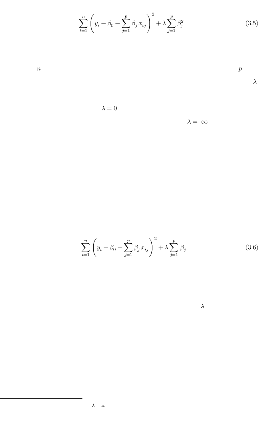
Equation 3.5 depicts the RSS and penalty term on the said regularization method.

The notation represents the total number of observations included in the model, while is the

number of candidate predictors. The essential factor in this equation is the tuning parameter ,

which controls the relative impact of the regression coefficient estimates

(James et al., 2013 p. 215). When , the penalty has no effect, and Ridge Regression

produces estimates similar to OLS estimates. However, as , the impact of

shrinkage penalty increases, and the coefficient estimates approach to zero (0) (Tiffin, 2016).

3.2.2.1.2. Least Absolute Shrinkage and Selection Operator

Another form of regularization method is the Least Absolute Shrinkage and

Selection Operator (LASSO). Similar to Ridge Regression, LASSO also includes a

penalty term to its RSS (Equation 3.6).

In contrast with the former regularization method, which only shrinks all of its

coefficients towards zero (0) but not set any of them exactly to zero (0), LASSO forces its

coefficients to be precisely equal to zero (0) when tuning the parameter is adequately large

(James et al., 2016).

40

Therefore, due to its substantial penalty, the main advantage of LASSO

over Ridge Regression is its ability to select important variables and produce a parsimonious

model with fewer predictors.

40

Except if the penalty of Ridge Regression is .

32

3.2.2.1.3. Elastic Net

Numerous studies also used Elastic Net (ENET) as their primary approach to

perform nowcasting to maximize the strengths of the two (2) aforementioned methods.

41

ENET is a form of regularization method that contains both properties of Ridge Regression and

LASSO (Equation 3.7).

In particular, this regularization method utilizes the penalty strength of Ridge Regression

and LASSO by selecting the best predictors to provide parsimonious models while still identifying

groups of correlated predictors. The respective weights of the two (2) penalties are determined

through the additional tuning parameter (Richardson et al., 2018).

3.2.2.2. Tree-Based Methods

Numerous studies also utilized tree-based methods as a primary approach to conduct

nowcasting. These studies particularly used Random Forest and Gradient Boosting Trees

because it has a strong resemblance with regularization methods, which are popular for their

capacity to address bias-variance tradeoff that provides an intuitive and easy-to-implement way

of modeling non-linear relationships.

However, in contrast with Ridge Regression, LASSO, and ENET, these methods are

considered non-parametric models that do not require the underlying relationship between the

dependent and independent variables (Fan, 2019). Tree-based methods involve stratifying or

segmenting the predictor space into a number of simple regions. Therefore, in order to make a

41

See the studies of Tiffin (2016), Richardson et al. (2018), and Tamara et al. (2020).

33

prediction for a given observation, tree-based methods utilize the mean or mode of training

observation in the region to which it belongs (James et al., 2013 p. 303).

3.2.2.2.1. Decision Tree

Decision Tree is the fundamental structure of any tree-based machine learning method,

which can be used for classification and regression problems (James et al., 2013; Fan, 2019).

Basically, this approach divides categorical (e.g., name, address) or continuous (e.g., level,

growth rate) data into two (2) classes in a systematic manner in order to reduce the prediction

error of the target variable of interest. This procedure is repeated until the number of training

samples at the branch exceeds the minimum node size (Figure 3.1). The algorithm, afterward,

makes the prediction by using the mean or mode of training observation in that particular region

(James et al., 2013).

Figure 3.1: Decision Tree Growing Process

(Recursive Binary Splitting of Two-Dimensional Feature Space)

Source: James et al. (2013)

34

3.2.2.2.2. Random Forest

One of the most well-known tree-based machine learning algorithms is the

Random Forest (RF). Mainly because this particular model is computationally simple to use,

does not require tuning of model parameters, and ideal for forecasting time series data with

relatively few observations (James et al., 2013).

RF is a machine learning algorithm that makes use of combinations of multiple

decision trees to formulate a comprehensive forecast. Notably, it modifies the approach of a

decision tree in order to minimize the problem of overfitting and maximize the information

content of the data by using subsamples of observations and predictions (Tiffin, 2016;

Bolhuis and Rayner, 2020). To perform this, RF uses bootstrap aggregation (also known as

bagging) in each decision tree using a random sample of observations in the training dataset.

This procedure is repeated number of times, and the results are averaged to reduce the overall

variance without increasing the bias of the dataset. It also uses random sampling in each split

to ensure that the multiple trees that go into the final collection are relatively diverse.

Using these approaches, RF generates an aggregate prediction that is strong and accurate

(Tiffin, 2016; Bolhuis and Rayner, 2020).

3.2.2.2.3. Gradient Boosted Trees

Gradient Boosted Trees (GBT) is another form of tree-based model that is often used

by numerous studies to conduct nowcasting. This is because of its powerful forecasting capability

to capture complex non-linear functions (Fan, 2019). However, compared with RF,

GBT is a machine learning algorithm that formulates sequential decision trees rather than

combinations to construct an aggregate forecast. This tree-based model does not involve

bootstrap sampling that RF conducts. GBT, instead, train an initial decision tree based on the

time-series data. It then uses the prediction errors from said decision tree to train a

second decision tree. The errors from the second decision tree are used to train the tree,

35

and so on. After the final iteration, the algorithm uses the summation of these predictions to

provide a final forecast (James et al., 2013; Bolhuis and Rayner, 2020).

3.3. Nowcast Evaluation Methodology

In this study, the performance of time series and machine learning algorithms are

evaluated based on their one-step-ahead (out-of-sample) nowcast. The models are trained over

an expanding window (also known as recursive) to estimate domestic liquidity growth from

January to December 2020 (Figure 3.2). For instance, for the first nowcast in January 2020,

the dataset used is based on January 2008 to December 2019. For the second nowcast in

February 2020, the dataset used is based on January 2008 to January 2020. This process is done

until the last out-of-sample period. Overall, there are twenty-four (24) generated nowcasts for

each time series and machine learning algorithms used in this research, with the end-month

nowcast being the principal prediction result.

42

Figure 3.2: Expanding Window Process

After the individual performance is evaluated, the forecast accuracy of each

model is gauged through their respective forecast errors such as Root Mean Square Error (RMSE)

42

Since there the data of target and input variables are unbalanced (e.g., monthly for target variable, daily/weekly for

input variable) problem. Averaging and interpolation are conducted to align of the data properly. This is further discussed in

Chapter 4: Research Data and Diagnostics.

36

(Equation 3.8) and Mean Absolute Error (MAE) (Equation 3.9). The RMSE and MAE of each

machine learning algorithm are compared against benchmark models (i.e., AR, DFM).

This method of comparison is performed to determine whether the nowcast results obtained from

the former are significantly superior to the latter methods or vice versa.

3.4. Research Tool

The R environment is the primary statistical software used in this study.

It is a well-known software environment for statistical computations, mathematical equations,

and data visualizations. In particular, this study highly utilized the capacity of R Studio to

perform the whole process of this research. This particular includes data integration,

data cleaning, model building, and statistical validation.

43

The R packages used in this study are listed in Annex A.

37

CHAPTER IV: DATA AND DIAGNOSTICS

CHAPTER V: EMPIRICAL RESULTS AND ANALYSIS

38

Chapter IV:

DATA AND DIAGNOSTICS

4.1. Primer

The activities performed to prepare datasets and enhance the overall performance of

benchmark and machine learning models used in this study are presented in this chapter.

In particular, each section presents the (1) dataset and variables, (2) averaging and interpolation

conducted, and (3) diagnostics and feature engineering efforts performed in this research.

4.2. Data

4.2.1. Target Variable

Driven by the objective and nature of this study, the dependent variable utilized is

the domestic liquidity in the Philippines. This monetary indicator represents the

total amount of money available in the economy of said country. The numerical figures

(i.e., level, growth rate) of domestic liquidity are acquired from the monthly

Depository Corporations Survey (DCS) that the Bangko Sentral ng Pilipinas (BSP) published

on its official website from January 2008 to December 2020.

44

,

45

Figure 3.1 depicts the level

(in million PHP) and year-on-year (YOY) growth rate (in percent), while Table 4.1 presents the

summary statistics of domestic liquidity in the Philippines.

4.2.2. Input Variables

Similar to previous studies that intend to formulate nowcasting models in order to

estimate recent developments of various macroeconomic indicators and transmission mechanisms

44

Official BSP Website: https://www.bsp.gov.ph.

45

To ensure that the data on domestic liquidity are not subject to any revisions, the last figure used in this study was as of

end-December 2020.

39

of policies through the use of machine learning algorithms, high-frequency data or information

are also used as independent variables in this study. These are comprised of numerous

high-frequency monetary, financial, and external sector indicators, which are used as

typical components to monitor or observe the growth of domestic liquidity.

Figure 4.1: Domestic Liquidity in the Philippines (January 2008-December 2020)

(a) Levels (in Million PHP); (b) Growth Rate (in Percent)

(a)

(b)

Table 4.1: Summary Statistics of Domestic Liquidity in the Philippines

MIN.

1ST QU.

MEDIAN

MEAN

3RD QU.

MAX

M3 (Level in PHP)

3,101,926

4,357,222

7,118,632

7,395,092

10,203,734

14,211,479

M3 (Growth %)

2.550

8.615

11.200

12.292

13.365

37.970

4.2.2.1. Monetary Indicators

The numerical data of monetary variables used in this study are formally requested from

the Department of Economic Statistics (DES) and obtained from the official website of the

BSP.

46

A formal request is made because daily figures of these variables are not published nor

shared publicly. Monetary indicators that are requested from the DES are the daily

(1) available reserves (i.e., required reserves, excess reserves) (2) reserve money

(i.e., currency-in-circulation, central bank liabilities). Meanwhile, the central bank (3) claims on

National Government (NG) and (4) claims on other sectors are obtained from the monthly

46

The DES is the technical arm of the BSP that generates monetary and economic statistics needed in the formulation and

implementation of monetary policy (2020 BSP Organization Primer, p. 25).

40

C

January 2008 to December 2020.

Table 4.2: List of Data

NO.

VARIABLE

TYPE

FREQ.

PUBLICATION DELAY

(DAYS AFTER REF. DATE)

1

Domestic Liquidity (M3) Growth

Target Variable

Monthly

30

2

M3 Growth (T-1)

Input Variable

Monthly

-

3

BSP Liabilities on National Government

Input Variable

Monthly

15

4

BSP Claims on Other Sectors

Input Variable

Monthly

15

5

Foreign Portfolio Investment (In)

Input Variable

Weekly

30

6

Foreign Portfolio Investment (Out)

Input Variable

Weekly

30

7

Available Reserves

Input Variable

Daily

1

8

Reserve Money

Input Variable

Daily

1

9

CBOE Volatility Index

Input Variable

Daily

1

10

Credit Default Swap

Input Variable

Daily

1

11

London Interbank Reference Rate

Input Variable

Daily

1

12

Singapore Interbank Reference Rate

Input Variable

Daily

1

13

Philippine Interbank Reference Rate

Input Variable

Daily

1

14

Philippine Government Bond Rate

Input Variable

Daily

1

15

BSP Discount Rate

Input Variable

Daily

1

16

Bank Savings Rate

Input Variable

Daily

1

17

Bank Prime Rate

Input Variable

Daily

1

18

Money Market Rate (Promissory Note)

Input Variable

Daily

1

19

Treasury Bill Rate

Input Variable

Daily

1

20

Interbank Call Rate

Input Variable

Daily

1

21

Philippine Peso per US Dollar (FOREX)

Input Variable

Daily

1

22

Weighted Monetary Operations Rate

Input Variable

Daily

1

4.2.2.2. Financial Indicators

Bloomberg. These are comprised of daily (1) Weighted Monetary Operations Rate (WMOR),

(2) BSP Discount Rate, (3) CBOE Volatility Index, (4) Credit Default Swap (CDS),

(5) London Interbank Offered Rates (LIBOR), (6) Singapore Interbank Offered Rates (SIBOR),

(7) Philippine Interbank Reference Rate (PHIREF), (8) Government Bond Rate,

41

(9) Interbank Call Loan Rate, (10) Bank Prime Rate, (11) Treasury Bill Rate, and

(12) Promissory Note Rate from January 2008 to December 2020.

4.2.2.3. External Indicators

Statistics for the external sector indicators are also obtained from Bloomberg.

However, the weekly figures of Foreign Portfolio Investment (FPI) are formally requested from

the International Operations Department (IOD) of the BSP.

47

Similar to the case of

available reserves and reserve money, its historical high-frequency values are not published nor

shared publicly. Other than the (1) FPI, (2) daily foreign exchange rate (i.e., Philippine Peso

per US Dollar) is also used as an external sector indicator in this study. The coverage of these

data is from January 2008 to December 2020.

4.2.2.4. Lagged Values of Domestic Liquidity

48

Although this study captures numerous monetary, financial, and external indicators as

input variables to predict the future movement of domestic liquidity in the Philippines,

other determinants that are not included in the dataset could also influence its growth.

To address this concern, lagged value of the domestic liquidity is also considered as an

input variable. The lagged values used in this study are of the target variable.

4.3. Averaging and Interpolation

Given that the main objective of this study is to provide useful and advance data or

information in order to minimize the usual approach in addressing different economic phenomena

and formulating policies based on outdated or lagged data, this study aims to nowcast

domestic liquidity in the Philippines on a bi-monthly basis, with the second nowcast being the

47

The IOD supports the BSP in maintaining the monetary stability and external sustainability through the management of

external debt, foreign investments, and other foreign exchange transactions (2020 BSP Organization Primer, p. 25).

48

Lagged values of domestic liquidity are only utilized under machine learning algorithms.

42

principal prediction result. This is to maximize the explanatory power of each high-frequency

input variable (i.e., variables with daily frequency). Aside from this, utilizing regressors with

high-frequency data typically solves the overfitting problem caused by the

observations).

However, based on the data publication release of each indicator (Table 4.2),

it can be observed that there is an unbalanced frequency problem. Standard regression models

require that the datasets should have the same level of granularity. Therefore, to align all of the

data correctly, averaging and interpolation are conducted in this study.

4.3.1. Averaging of High-Frequency Variables

Data averaging is performed on variables with a daily and weekly frequency.

The input variables (e.g., monetary, financial indicators) with daily frequency are aggregated

and averaged into two (2) numerical values in a month. The first value is the average of

1st until the 15th day of the month, while the other half is the mean of 16th until the last day

of the month (e.g., available reserves data from 1 to 15 January and 16 to 31 January are

averaged, respectively). On the other hand, explanatory variables with weekly frequency are

averaged based on the first and second week as well as third and fourth-week data release,

respectively (e.g., first- and second-week data of foreign portfolio investment are averaged).

4.3.2. Interpolation of Low-Frequency Variables

Data interpolation is conducted on the variables with low frequency (i.e., monthly),

such as domestic liquidity, BSP liabilities on NG, and BSP claims on other sectors.

Since these are published on a monthly basis, their official data are categorized as the

month-end growth rate. The data points between each period of averaged input variable data

(e.g., mid-month data) are considered missing values and interpolated using a

spline interpolation method, which is commonly used for non-linear data estimation.

43

4.4. Diagnostics and Feature Engineering

The raw dataset is refined to improve the performance of time series and machine

learning algorithms used in this study. In particular, data of target and input variables are

(1) seasonally adjusted, (2) log-transformed, and (3) individually assessed if they are stationary.

4.4.1. Seasonal Adjustment

Since most published data in the Philippines are not seasonally adjusted,

data of domestic liquidity and most input variables used in this study are deseasonalized

accordingly. This includes data that were requested from the DES and IOD as well as the other

statistics obtained from the official website of the BSP and Bloomberg

(e.g., BSP liabilities to NG, BSP discount rate). The aforementioned correction was performed

to ensure that estimates from the time series and machine learning models are accurate since

seasonal components (e.g., holidays) are not present in each model simulation.

4.4.2. Logarithmic Transformation

The normality of data is also an important factor in economic and statistical modeling.

Given that most real-life datasets do not always follow a normal distribution, they are often

skewed, which makes the empirical results or analysis spurious. Therefore, to address this

concern, the numerical figures of target and input variables in this study are transformed based

on their respective logarithmic equivalent.

49

4.4.3. Stationarity

In order to develop an accurate or precise forecasting model, it is crucial to establish that

the time series data of each indicator is stationary. This is mainly performed in order to ensure

49

If the data of a variable is an index or growth rate, it is not transformed to its logarithmic equivalent.

44

that the statistical properties of each time series do not change over time.

In this study, the stationarity of target and input variables are verified through the

Augmented Dickey-Fuller (ADF) and Philipps-Perron (PP) tests.

Based on the conducted unit root tests, the level, growth rate, or logarithmic equivalent

of domestic liquidity and input variables are non-stationary (Table 4.3).

50

This is because their

individual p-value is greater than the five (5) percent significance level (except for central bank

liabilities to NG). However, when transformed in their respective first difference, ADF and

PP tests showed that these variables are stationary. Therefore, to formulate a nowcasting model

to estimate domestic liquidity growth in the Philippines, the first difference values of target and

input variables (except for BSP Liabilities to NG) are used in this study.

51

Table 4.3: Unit Root Tests for Domestic Liquidity in the Philippines

VARIABLE

TEST

LEVEL OF SIG.

P-VALUE

(LEVEL/GROWTH/LOG)

P-VALUE

(FIRST DIFF.)

Domestic Liquidity (M3)

ADF

PP

0.05

0.14

0.61

0.01

Figure 4.2: Domestic Liquidity in the Philippines (January 2008 December 2020)

(a) Growth Rate (in %); (b) Growth Rate (in %, First Difference)

(a)

(b)

50

See Annex B for the individual ADF and PP test result of input variables.

51

For univariate models, the process of obtaining the first difference values of target variable is conducted within the ARIMA and

RW process. For DFM and machine learning models (i.e., regularization, tree-based methods), data of target and input variables

are transformed by their first difference prior model simulation.

45

Figure 4.3: Research Workflow Diagram

46

Chapter V:

EMPIRICAL RESULTS AND ANALYSIS

5.1. Primer

In this chapter, results of the simulated nowcasts using time series and

machine learning algorithms are presented. The sections of this chapter mainly discuss the

(1) calibration method performed in each model, (2) individual performance of

benchmark and machine learning models through the expanding window validation, and

(3) critical high-frequency indicators (i.e., monetary, financial, external sectors) that are

considered important to accurately nowcast the real-time growth of domestic liquidity in the

Philippines.

5.2. Calibration and Nowcast Results

5.2.1. One-Step-Ahead (Out-of-Sample) via Expanding Window

Since the main objective of this study is to accurately determine the growth of

domestic liquidity in the short-run, one-step-ahead (out-of-sample) nowcasts are performed.

This particular approach is preferred compared with multi-step-ahead (out-of-sample) estimates

because of two (2) primary underlying reasons. The first reason is to ensure that the

recent numerical figures of target and input variables are part of the structure and characteristics

of the training datasets. The second reason is to maximize the forecasting ability of

time series models, specifically Autoregressive Integrated Moving Average (ARIMA) and

Random Walk. Mainly because these univariate models place heavier emphasis on the recent

past rather than the distant past in conducting a forecast. Therefore, to appropriately compare

the accuracy of benchmark models vis-à-vis machine learning algorithms, their respective

one-step-ahead (out-of-sample) nowcasts should be considered one of the bases of evaluation.

47

It is also crucial to determine the precision consistency of simulated nowcasting models.

Therefore, the benchmark and machine learning models are trained over an expanding window

(also known as recursive method) to provide a series of one-step-ahead (out-of-sample) nowcast.

The bi-monthly dataset covering thirteen (13) years from 2008 to 2020 is divided into

twelve (12) different training and test datasets to perform the said approach.

The first training dataset covers the numerical figures of the target and input variables from

January 2008 to December 2019. Meanwhile, its corresponding test dataset is comprised of the

numerical statistics of target and input variables as of January 2020. This process is

accomplished until the test dataset covers the numerical figures of the target and input variables

as of December 2020. Overall, there are twenty-four (24) generated nowcasts for each

time series model and machine learning algorithm, with the end-month one-step-ahead

(out-of-sample) nowcast being the principal prediction result. The estimates of benchmark

models and machine learning algorithms under the said approach are then evaluated

individually and collectively based on their Root Mean Squared Error (RMSE) and

Mean Absolute Error (MAE).

5.2.2. Autoregressive Models

5.2.2.1. Model Calibration

In this study, the trained models under univariate or Autoregressive (AR) methods are

simulated based on three (3) different approaches. The first simulated model has the

parameters (0,1,0) of an ARIMA structure, otherwise known as Random Walk (RW).

This model was formulated because the time series data of domestic liquidity shows an

irregular growth as found in the conducted Augmented Dickey-Fuller (ADF) and

Philipps-Perron (PP) tests. To address this concern, one of the best strategies is to predict the

change that occurs from one period to the next rather than directly predicting the level of the

series at each period. In other words, it is essential to observe the first difference of the

time series to monitor if there are predictable patterns that can be determined (Nau, 2014).

48

The second univariate model simulated has the parameters (4,1,1) of an ARIMA Model.

This is formulated since the Partial Autocorrelation Function (PACF) as well as

Akaike Information Criterion (AIC) suggest that four (4) autoregressive (AR) lags should be

considered to forecast domestic liquidity in the Philippines (Figure 5.1). It is also simulated

because the time series data of said monetary indicator was found to be non-stationary.

Hence, in some cases of non-stationary time series, it is essential to use the average of the

last few observations to filter out the noise and accurately estimate the local mean (Nau, 2014).

Figure 5.1: ACF and PACF of Domestic Liquidity Growth in the Philippines (Seasonally Adjusted)

(a) ACF of M3 (Seasonally Adjusted); (b) PACF of M3 (Seasonally Adjusted)

(a)

(b)

Figure 5.2: Residual Plot for ARIMA (4,1,1)

52

The red-colored line under the ACF of ARIMA(4,1,1) indicates that a seasonal lag should be included in overall model.

49

Lastly, the parameters of the third univariate model are established based on the

built-in function of the statistical software, R Studio. The decision to use this automated process

is due to the seasonal lag that was found to be relevant under the

Autocorrelation Function (ACF) of ARIMA (4,1,1) (Figure 5.2). For this reason,

the third univariate model utilized in this study is a seasonal ARIMA (SARIMA) with

parameters based on the characteristics of the twelve (12) training datasets.

53

5.2.2.2. Nowcast Results

Figure 5.3: Autoregressive Model Nowcasts vs. Actual M3 Growth (January to December 2020)

(In Percent, Year-on-Year Seasonally Adjusted)

Based on the three (3) univariate models conducted, results indicate that their respective

one-step-ahead (out-of-sample) nowcasts from January to December 2020 strongly adhere to the

overall trend of domestic liquidity growth in the Philippines (Figure 5.3).

The ARIMA, RW, and auto-SARIMA models provided decent estimates in the months where

the growth of said monetary indicator (i.e., March, April, May) suddenly expand due to the

53

The parameters under auto-SARIMA models can be different from January to December 2020. This is because R Studio selects

the optimal lag orders to forecast domestic liquidity in each time period. For example, univariate model to nowcast January 2020

has the parameters ARIMA(2,1,4)(1,0,1) while for February 2020 the model has the parameters of ARIMA(5,1,1)(1,0,1).

50

increase in the borrowings of the National Government (NG) to minimize the negative impact

of Coronavirus Disease 2019 (COVID-19) pandemic in the economy of said country.

54

However, by comparing their respective monthly forecast errors, it can be observed that

no specific univariate model can accurately estimate the growth of domestic liquidity throughout

the expanding window. Tables 5.1 and 5.2 displayed that auto-SARIMA provided the highest

number of months with low RMSE and MAE (i.e., March, May, September, November,

December). This was followed by Random Walk (i.e., January, February, June, July) and

ARIMA (i.e., April, August, October), respectively. The accurate nowcasts from auto-SARIMA

are expected since the statistical software R Studio designates its parameters.

Table 5.1: RMSE of Autoregressive Models

55

M1

M2

M3

M4

M5

M6

M7

M8

M9

M10

M11

M12

OVR.

ARIMA

0.716

1.422

0.936

1.663

0.196

1.636

0.474

0.102

0.649

0.117

0.452

0.577

0.917

R. Walk

0.288

0.722

1.470

2.415

0.434

1.095

0.425

0.403

0.669

0.199

0.880

0.895

1.016

A. SARIMA

1.622

1.879

0.556

1.986

0.134

1.535

0.702

0.428

0.299

0.174

0.222

0.057

1.066

Table 5.2: MAE of Autoregressive Models

M1

M2

M3

M4

M5

M6

M7

M8

M9

M10

M11

M12

OVR.

ARIMA

0.715

1.395

0.762

1.537

0.194

1.527

0.467

0.088

0.544

0.106

0.389

0.537

0.688

R. Walk

0.273

0.669

1.319

2.327

0.428

0.996

0.416

0.380

0.543

0.149

0.825

0.862

0.766

A. SARIMA

1.609

1.801

0.405

1.854

0.134

1.411

0.650

0.355

0.244

0.162

0.194

0.050

0.739

The overall forecast errors of the three (3) univariate models, on the other hand,

provided different results to the aforementioned statement. Based on their overall RMSE and

MAE, it can be observed that ARIMA (4,1,1) is the most appropriate univariate time series

model to estimate the growth of domestic liquidity. This is because the said model registered

the most accurate overall nowcasts with RMSE of 0.917 and MAE of 0.688.

54

https://www.bsp.gov.ph/SitePages/MediaAndResearch/MediaDisp.aspx?ItemId=5297

55

M1 to M12 refers to the months included in the expanding window validation (e.g., January, February 2020).

51

Both of these indicators are lower compared to forecast errors registered by

RW (1.016 and 0.766) and auto-SARIMA (1.066 and 0.739), respectively

(Tables 5.1 and 5.2).

5.2.3. Dynamic Factor Model

5.2.3.1. Model Calibration

Dynamic Factor Model (DFM) is also utilized in this study to systematically include the

wide range of high-frequency monetary, financial, and external sector indicators as

input variables. Hence, this study followed the methodology used by

Mariano and Ozmucur (2020) in implementing the said approach, wherein:

(1) the number of indicators is reduced through factor analysis; (2) factors identified are applied

under a Vector Autoregressive (VAR) framework; and (3) predicted values from the

aforementioned are then used to nowcast the target variable.

Figure 5.4: Eigenvalues of Input Variables via Factor Analysis

By performing factor analysis, three (3) determinants were extracted from the initial

twenty (20) input variables using the method of maximum likelihood. The decision to use the

aforementioned factors was strongly based on each indicator's eigenvalues and

52

cumulative variance.

56

Figure 5.4 indicates that factors one (1) to three (3)

(i.e., first three (3) blue points) have larger eigenvalues in contrast to the remaining

seventeen (17) factors. Although using a higher number of factors is still acceptable,

the first three (3) factors already explain the sixty-four (64) percent of the variance in the

twenty (20) different monetary, financial, and external sector indicators used in this study.

57

After the aforementioned process, the three (3) factors identified are then utilized under

a VAR framework in order to complete the method of estimating the growth of

domestic liquidity in the Philippines. The optimal lags for this model are selected based on the

AIC and Hannan-Quinn (HQ) Information Criterion. Based on these selection criteria,

five (5) autoregressive lags should be considered under the twelve (12) training models to

determine the estimates from January to December 2020.

5.2.3.2. Nowcast Results

Compared with the three (3) univariate models conducted, DFM, as a nowcasting model,

provides inconsistent estimates on the overall movement of domestic liquidity in the

first semester of 2020. The one-step-ahead (out-of-sample) nowcasts of said model, in particular,

did not precisely estimate the expansion of domestic liquidity due to the sharp increase in the

borrowings and deposits of NG to the central bank that took effect last March to May 2020

(Figure 5.5).

On the contrary, the DFM provides more accurate results in the latter half of the year.

It can be observed in Tables 5.3 and 5.4 that the monthly forecast errors of the said model are

relatively lower than those under ARIMA, Random Walk, and auto-SARIMA, particularly from

August to December 2020. This outcome is also noticed from the overall forecast errors of DFM.

The said multivariate model only conveyed an overall RMSE and MAE of 0.825 and 0.619,

56

Eigenvalues refers to the total amount of variance that can be explained by a given principal component/factor.

57

Sixty (60) to sixty-five (65) percent of variance is the common figure used in economic analysis (Mariano and Ozmucur, 2020).

53

respectively. These forecast errors are relatively lower than the overall RMSE and MAE

displayed by the univariate models (Figure 5.6).

Figure 5.5: DFM Nowcasts vs. Actual M3 Growth (January to December 2020)

(In Percent Difference, Seasonally Adjusted)

Table 5.3: RMSE of DFM

M1

M2

M3

M4

M5

M6

M7

M8

M9

M10

M11

M12

OVR.

DFM

0.557

1.093

0.565

1.458

0.247

1.678

0.965

0.184

0.513

0.182

0.078

0.267

0.825

Table 5.4: MAE of DFM

M1

M2

M3

M4

M5

M6

M7

M8

M9

M10

M11

M12

OVR.

DFM

0.526

1.091

0.509

1.446

0.237

1.649

0.918

0.138

0.452

0.136

0.077

0.246

0.619

Figure 5.6: Overall (a) RMSE and (b) MAE of Autoregressive Models and DFM

(a)

(b)

54

5.2.4. Machine Learning Models

Before using any machine learning algorithms, it is common to validate their respective

stability using the cross-validation method. This is to ensure that the models can strongly

regulate the bias-variance tradeoff and accurately provide new estimates based on the training

or historical data (James et al., 2013). In this study, therefore, the aforementioned approach is

performed before conducting a series of recursive nowcasts on the growth of domestic liquidity

in the Philippines via regularization (i.e., Ridge Regression, Least Absolute Shrinkage and

Selection Operator, Elastic Net) and tree-based (i.e., Random Forest, Gradient Boosted Trees)

methods.

Although there are various methods to cross-validate machine learning methods

(e.g., holdout method, stratified K-Fold cross-validation), this study particularly utilized

(1) K-Fold cross-validation and (2) leave-one-out cross-validation methods for the

twelve (12) training datasets of target and input variables. Specifically, training datasets

under Ridge Regression, Least Absolute Shrinkage and Selection Operator (LASSO),

Elastic Net (ENET), and Gradient Boosted Trees (GBT) are tuned based on a

Ten (10)-Fold cross-validation. In contrast, training datasets under Random Forest (RF) are

calibrated based on their out-of-bag (OOB) scores.

58

,

59

5.2.4.1. Regularization Methods

5.2.4.1.1. Model Calibration

The optimal shrinkage penalty for each algorithm under regularization methods is

determined based on a ten (10) fold cross-validation method. Under this approach, twelve (12)

different values of the said parameter are determined since twelve (12) training datasets are used

in each regularization algorithm. In order words, the value of shrinkage penalty is specifically

58

10-Fold cross-validation is the standard cross-validation technique used in machine learning exercises.

59

OOB is virtually equivalent to leave-one-out cross validation (James et al., 2013).

55

tailored based on the attributes of the training datasets and the norm of regularization

(i.e., Ridge Regression, LASSO, ENET). Figure 5.6 explicitly presents this scenario.

It shows that the optimal shrinkage penalty for estimating the domestic liquidity for

January 2020 has a different value than the optimal shrinkage penalty to predict the said

monetary indicator for February 2020. In particular, Panel A shows that the former has an

optimal shrinkage penalty value of 0.772, while Panel B presents that the latter has an

optimal shrinkage penalty value of 1.012.

60

Figure 5.7: Optimal Shrinkage Penalty via Ridge Regularization (January and February 2020)

(a) Training Dataset to Estimate M3 Jan. 2020; (b) Training Dataset to Estimate M3 Feb. 2020

(a)

(b)

5.2.4.1.2. Nowcast Results

After being calibrated based on their specific shrinkage penalty, models under

regularization methods then estimate domestic liquidity growth using the test datasets from

January to December 2020. The result from recursive nowcasts displayed that

Ridge Regression, LASSO, and ENET provide more consistent and accurate projections

compared to the estimates provided by the benchmark models conducted in this study.

Particularly, monthly estimates based on the three (3) machine learning algorithms significantly

have lower forecast errors compared to the individual nowcasts stipulated by the

benchmark models used in this study, such as ARIMA, RW, auto-SARIMA, and DFM

60

See Annex C to E for the complete list of optimal shrinkage penalty for each training dataset via regularization methods.

56

(Tables 5.5 and 5.6), except for September and October 2020 (Figure 5.8). The Ridge Regression,

LASSO, and ENET also provided accurate nowcasts on the unexpected increase in the growth

of domestic liquidity due to the increase in NG borrowings and deposits to BSP in March and

April 2020 (Tables 5.5 and 5.6).

The aforementioned result can also be observed from the overall forecast errors of

the three (3) machine learning algorithms. Mainly because Ridge Regression, LASSO, and ENET

have provided low overall RMSE and MAE in comparison with the overall forecast errors of

ARIMA (0.917 and 0.688), Random Walk (1.016 and 0.766), auto-SARIMA (1.066 and 0.739),

and DFM (0.825 and 0.619) (Figure 5.9).

Figure 5.8: Regularization Method Nowcasts vs. Actual M3 Growth (January to December 2020)

(In Percent Difference, Seasonally Adjusted)

Table 5.5: RMSE of Ridge Regression, LASSO, and ENET

M1

M2

M3

M4

M5

M6

M7

M8

M9

M10

M11

M12

OVR.

Ridge

0.292

0.372

0.928

1.163

0.173

0.258

0.261

0.248

0.596

0.449

0.123

0.349

0.529

LASSO

0.264

0.237

0.964

1.348

0.046

0.185

0.179

0.215

0.621

0.416

0.115

0.286

0.551

ENET

0.262

0.259

0.973

1.328

0.048

0.199

0.206

0.187

0.631

0.390

0.099

0.291

0.549

However, by comparing the three (3) models under the regularization method,

it can be observed that LASSO is the most accurate machine learning model to nowcast the

57

growth of domestic liquidity in the Philippines. Mainly because the said machine learning

algorithm provided the highest number of months with low forecast error estimates from

January to December 2020. Despite the strong monthly accuracy of LASSO, however,

Ridge Regression and ENET registered the most accurate overall estimates. This is because the

former notably provided an RMSE of 0.529, while the latter registered an MAE of 0.391

which were both lower compared to the overall forecast error of LASSO (Tables 5.5 and 5.6).

Table 5.6: MAE of Ridge Regression, LASSO, and ENET

M1

M2

M3

M4

M5

M6

M7

M8

M9

M10

M11

M12

OVR.

Ridge

0.292

0.364

0.887

1.136

0.156

0.245

0.259

0.209

0.596

0.325

0.116

0.345

0.411

LASSO

0.257

0.234

0.909

1.340

0.040

0.182

0.179

0.202

0.620

0.345

0.114

0.281

0.392

ENET

0.255

0.257

0.916

1.321

0.036

0.196

0.206

0.171

0.631

0.318

0.099

0.286

0.391

Figure 5.9: Overall (a) RMSE and (b) MAE of Benchmark Models and Regularization Methods

(a)

(b)

5.2.4.2. Tree-Based Methods

5.2.4.2.1. Model Calibration

Similar to regularization methods, RF and GBT are tuned under the cross-validation

method to provide accurate estimates on domestic liquidity growth from January to

December 2020. The methods used to calibrate these two (2) algorithms are OOB scores and

10-Fold cross-validation. By doing this, the twelve (12) training datasets under

58

RF and GBT individually have an optimal number of variables randomly sampled as candidates

at each split and the number of trees to grow, respectively.

The results of these calibration techniques further elaborate this discussion.

Figure 5.10 depicts the OOB errors of the training datasets under RF for January and

February 2020. Panel A shows that five (5) indicators are already sufficient to estimate domestic

liquidity growth for January 2020 since it has the lowest OOB error of 1.018. On the other hand,

Panel B indicates that ten (10) indicators are necessary to accurately nowcast the growth of said

monetary indicator for February 2020 because it registered the lowest OOB error of 1.014.

Figure 5.10: OOB Error of Training Datasets via Random Forest

61

(a) Training Dataset to Estimate M3 Jan. 2020; (b) Training Dataset to Estimate M3 Feb. 2020

(a)

(b)

Figure 5.11: Optimal Number of Trees via Gradient Boosted Trees

62

(a) Training Dataset to Estimate M3 Jan. 2020; (b) Training Dataset to Estimate M3 Feb. 2020

(a)

(b)

61

See Annex F for the complete list of OOB errors for each training dataset via Random Forest.

62

See Annex G for the complete list of the optimal number of trees for each training dataset via Gradient Boosted Trees.

59

Meanwhile, Figure 5.11 illustrates the optimal number of trees that should be considered

to accurately nowcast the growth of domestic liquidity under GBT. Panel A presents

that sixty-seven (67) iterations are necessary to provide a precise estimate of

domestic liquidity growth for January 2020. On the other hand, Panel B depicts that fifteen (15)

iterations are already sufficient for the GBT model to accurately nowcast domestic liquidity

growth for February 2020.

5.2.4.2.2. Nowcast Results

Similar to the results under regularization methods, utilizing RF and GBT as

primary nowcasting models also stipulates more consistent and accurate estimates in contrast

with the benchmark models conducted in this study. The monthly forecast errors of the

two (2) machine learning models are also significantly lower than those under ARIMA, RW,

auto-SARIMA, and DFM, except for the nowcast result of RF in September 2020.

Based on the recursive nowcasts, it can also be found that RF and GBT provide decent

projections on the months (e.g., March, April, May) where the growth of domestic liquidity

unexpectedly expands due to the increased borrowings and deposits of NG to the BSP

(Tables 5.7 and 5.8).

Figure 5.12: Tree-Based Method Nowcasts vs. Actual M3 Growth (January to December 2020)

(In Percent Difference, Seasonally Adjusted)

60

Aside from their robust monthly estimates, the overall nowcasts of RF and GBT based

on the expanding window also registered a lower set of RMSE and MAE.

The result indicates that RF only displayed forecast errors of 0.595 and 0.432 for RMSE and

MAE, respectively. Meanwhile, GBT provided marginal RMSE of 0.632 and MAE of 0.469.

The figures mentioned are significantly lower than the overall forecast errors provided by the

univariate and multivariate models performed in this study (Figure 5.13).

Table 5.7: RMSE of RF and GBT

M1

M2

M3

M4

M5

M6

M7

M8

M9

M10

M11

M12

OVR.

RF

0.346

0.389

0.879

1.455

0.265

0.208

0.167

0.265

0.855

0.203

0.077

0.307

0.595

GBT

0.180

0.686

0.986

1.536

0.060

0.495

0.305

0.241

0.636

0.248

0.201

0.216

0.632

Table 5.8: MAE of RF and GBT

M1

M2

M3

M4

M5

M6

M7

M8

M9

M10

M11

M12

OVR.

RF

0.345

0.377

0.830

1.454

0.242

0.201

0.140

0.235

0.852

0.147

0.058

0.307

0.432

GBT

0.179

0.684

0.972

1.530

0.060

0.490

0.243

0.201

0.636

0.218

0.200

0.215

0.469

Figure 5.13: Overall (a) RMSE and (b) MAE of Benchmark Models vs. Tree-Based Methods

(a)

(b)

Based on the aforementioned discussion, it can also be established that RF is the most

accurate tree-based model to nowcast the growth of domestic liquidity despite having an

inaccurate estimate in September 2020. Mainly because the said model notably provided the

highest number of months with precise estimates from January to December 2020.

61

This includes the nowcasts for January, February, March, April, June, July, November, and

December 2020 (Tables 5.7 and 5.8).

5.3. Further Analysis

5.3.1. Variable Importance

One of the main advantages of using machine learning algorithms in economic nowcasting

is their strong capability to identify critical factors that could comprehensively explain the

movement or growth of a particular macroeconomic indicator and scenario. Numerous studies

have already established that these algorithms can formulate quantitative models

with accurate estimates despite using a limited number of indicators.

63

Among the machine learning models that specifically have this ability are regularization and

tree-based methods, such as LASSO, ENET, RF, and GBT.

64

5.3.1.1. LASSO and ENET

Based on the recursive nowcasts conducted by LASSO and ENET from

January and February 2020, it was found that (1) foreign exchange rate (FOREX),

(2) inflow of FPI, (3) LIBOR, (4) bank savings rate, (5) NG deposits to the central bank, and

(6) liabilities of other sectors to the central bank are among the critical indicators that should

be considered in estimating the growth of domestic liquidity in the Philippines.

Mainly because among the twenty-one (21) indicators used as input variables, these are the

consistent determinants under LASSO and ENET that do not stipulate zero coefficients

in January and February 2020 (Table 5.9).

65

63

See the studies of Cepni et al. (2018), Richardson et al. (2018), Ferrara and Simoni (2019), and Tamara et al. (2020).

64

See Chapter 3 for the comprehensive discussion on these models.

65

Other months identified BSP Discount Rate, Bank Savings Rate, and WMOR as important indicators (See Annex H and I).

62

5.3.1.2. Random Forest and Gradient Boosted Trees

The critical indicators identified under RF and GBT are similar to the input variables

that LASSO and ENET provided. However, the main difference is that both of the tree-based

methods used in this study have identified that lagged values of the target variable,

as an input variable, are also crucial to provide an accurate estimate of domestic liquidity growth

in the Philippines. In particular, Figures 5.14 and 5.15 indicate that (1) M3 ,

(2) liabilities of other sectors to the central bank (OSC), and (3) NG deposits to the central

bank (NGD) are by far the three (3) most important variables that should be considered in

estimating the growth of domestic liquidity in the Philippines.

Table 5.9: Variable Coefficients via LASSO and ENET from (January-February 2020)

NO.

VARIABLE

LASSO

(JAN. 2020)

LASSO

(FEB. 2020)

ENET

(JAN. 2020)

ENET

(FEB. 2020)

-

Intercept

0.016

0.015

0.016

0.015

1

M3 Growth (T-1)

-

2

BSP Liabilities on National Government

-0.015

-0.014

3

BSP Claims on Other Sectors

0.235

0.216

4

Foreign Portfolio Investment (In)

-0.003

-0.004

-0.010

5

Foreign Portfolio Investment (Out)

-

6

Available Reserves

-

7

Reserve Money

-

8

CBOE Volatility Index

-

9

Credit Default Swap

-

10

London Interbank Reference Rate

0.111

0.114

0.097

0.100

11

Singapore Interbank Reference Rate

-

12

Philippine Interbank Reference Rate

-

13

Philippine Government Bond Rate

-

14

BSP Discount Rate

-

15

Bank Savings Rate

-0.103

-0.110

-0.080

-0.087

16

Bank Prime Rate

-

17

Money Market Rate (Promissory Note)

-

18

Treasury Bill Rate

-

19

Interbank Call Rate

-

20

Philippine Peso per US Dollar (FOREX)

0.124

0.111

0.119

21

Weighted Monetary Operations Rate

-

63

Figure 5.14: Node Impurity via Random Forest

Figure 5.15: Variable Importance Plot via Gradient Boosted Trees

64

CHAPTER VI: CONCLUSION

CHAPTER VII: RECOMMENDATION

65

Chapter VI:

CONCLUSION

6.1. Summary and Conclusion

Domestic liquidity (also known as broad money) is defined as the sum of all

liquid financial instruments held by money-holding sectors that are used as a

medium of exchange in an economy (IMF, 2016). The changes in the overall growth of this

monetary indicator are among the most important dynamics that numerous central banks are

closely monitoring. This is because of its property of being an essential element to the

overall transmission mechanism of monetary policy, particularly the impact of

money supply expansion or contraction on aggregate demand, interest rates, inflation, and

overall economic growth (Mankiw, n.d.).

In the Philippines, data on domestic liquidity is used as a primary component

to formulate monetary policy and utilized as a leading indicator to observe

price and financial stability. However, similar to the concerns regarding the delayed publication

of data or statistical indicators generated by most government offices, data on domestic liquidity

in the said country also suffers from series of lags and revisions. Due to this predicament,

policymakers in the Central Bank of the Philippines or Bangko Sentral ng Pilipinas (BSP)

typically formulate monetary policies and address different economic phenomena (e.g., inflation,

business cycle) using its outdated or lagged values.

The concept of short-

methodologies utilized by numerous institutions (e.g., International Financial Institutions (IFIs),

central banks) to address the aforementioned issues in data publication. This approach,

at present, also became prevalent because of the emergence of the use of big data and

machine learning. These approaches augment the overall process in providing a solution for the

difficulty in producing data on a real-time basis. Mainly because the two (2) methodologies

provide complementary information concerning the macroeconomic data that government offices

66

usually published and stipulate accurate estimates using an immense amount of data or

information, respectively (Hassani and Silva, 2015; Richardson et al., 2018).

Drawing upon this background, the concept of nowcasting using different

machine learning algorithms is utilized in this study to address the aforementioned issues,

particularly in addressing the lag data release on domestic liquidity in the Philippines.

This objective intends to formulate an accurate quantitative model that the BSP can sustainably

use to estimate the short-run growth of said monetary indicator. Therefore, five (5) popular

machine learning algorithms under regularization methods (i.e., Ridge Regression,

Least Absolute Shrinkage and Selection Operator (LASSO), Elastic Net (ENET)) and

tree-based method (i.e., Random Forest (RF), Gradient Boosted Trees (GBT)) using different

high-frequency monetary, financial, and external sector indicators from January 2008 to

December 2020 are performed to support the objective of this study. The performances of these

algorithms are then compared against traditional time series models such as Autoregressive (AR)

and Dynamic Factor Models (DFM). In particular, their respective one-step-ahead

(out-of-sample) nowcasts under an expanding window process are evaluated based on monthly

and overall Root Mean Squared Error (RMSE) and Mean Absolute Error (MAE).

The results demonstrate that machine learning algorithms provide more accurate

estimates than the benchmark models used in this study. Mainly because the said approaches

registered consistent monthly estimates with low forecast errors. Tables 6.1 and 6.2 depict that

the nowcasts of machine learning algorithms are more accurate than the estimates provided by

AR models and DFM. It can also be observed that the overall RMSE and MAE of

all machine learning models used in this study are more accurate than the benchmark models.

These algorithms, in addition, registered precise estimates on the months (i.e., March, April,

May) where domestic liquidity growth suddenly expand (e.g., increased borrowings and deposits

of the National Government (NG) to BSP) due to the impact of the Coronavirus Disease 2019

(COVID-19) in the Philippines. Based on these outcomes, it can be concluded that both

regularization and tree-based machine learning algorithms could be used as alternative models

to estimate the growth of domestic liquidity in the Philippines.

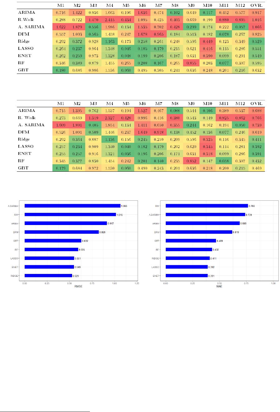
67

Table 6.1: RMSE of Benchmark and Machine Learning Models (Summary)

66

Table 6.2: MAE of Benchmark and Machine Learning Models (Summary)

Figure 6.1: Overall Forecast Errors of Benchmark and Machine Learning Models

(a)

(b)

However, among the quantitative models, LASSO and RF provided the highest number

of months (i.e., three/four out of twelve) with at least low forecast error from January to

December 2020. The Ridge Regression and ENET, on the other hand, registered the lowest

overall RMSE and MAE with 0.529 and 0.391, respectively (Figure 6.1). These results provide

a shred of solid evidence that nowcasting through regularization methods is the most appropriate

approach to nowcast the said monetary indicator using machine learning algorithms.

66

The red-colored cells represent high forecast errors, while yellow- and green-colored cells are moderate to low forecast errors.

68

Using machine learning algorithms as a primary nowcasting approach also provides

substantial advantages against traditional time series models such as AR and DFM.

This is because the regularization and tree-based machine learning models can filter out or

identify important indicators that could stipulate parsimonious nowcasting models with precise

results. The results of the conducted recursive nowcasts based on LASSO, ENET, Random

Forest, and Gradient Boosted Trees indicate that (1) BSP Liabilities on National Government,

(2) BSP Claims on Other Sectors, (3) Foreign Exchange Rate, and (4) Lagged Values of M3 are

among the critical indicators that should be considered in estimating the growth of domestic

liquidity in the Philippines.

69

Chapter VII:

RECOMMENDATION

7.1. Potential Actions

Since the results of the conducted recursive nowcasting established the superiority of

different machine learning algorithms in estimating domestic liquidity growth in the Philippines,

this study highly recommends that the departments (i.e., statistics, research departments) under

the Central Bank of the Philippines or Bangko Sentral ng Pilipinas (BSP) should adopt and

utilize the concept of big data and machine learning. Implementing these concepts could support

the objective of the BSP in conveying data-based monetary policy in the country.

Furthermore, the additional data or information that can be gathered by the

different departments in the said institution could further improve the individual and

overall accuracy of each machine learning algorithm used in this study.

However, although this cannot be guaranteed, it is always better to calibrate models using an

immense amount of data or information than operating with a limited number of indicators.

Among the possible determinants that the BSP could explore and collect over time are

high-frequency (e.g., daily, weekly) unconventional data or information regarding the

credit condition of the Philippine Banking System (PBS) and the overall demand of the general

public to hold or forego money. Mainly because domestic credit which is composed of

loans outstanding for production and household consumption is considered a significant

contributor to the monthly change in domestic liquidity in the Philippines.

The study also recommends a regular and sustainable way of accumulating other

statistics related to the critical indicators identified in this study. This could include

high-frequency data or information regarding (1) debt securities issued by the

National Government (NG) and the BSP, (2) amount of loans granted by the BSP to

Other Depository Corporations (ODCs), (3) amount of loans granted by the BSP to

70

Other Sectors (e.g., Other Financial Corporations), and (4) New Effective Exchange Rate

(NEER) Indices of Philippine Peso.

7.2. Suggestions for Future Research

As mentioned in the previous chapters, this study has limitations in formulating the

different nowcasting models using time series and machine learning algorithms.

Therefore, the following are suggested to enhance the results and comprehensiveness of this

research:

a. It is recommended to combine the different machine learning algorithms with

low monthly and overall forecast errors. This approach (known as the

ensemble method) is performed to have a single model that contains the strength of

each algorithm. Studies of Tiffin (2016), Richardson et al. (2018),

Mariano and Ozmucur (2020), and Tamara et al. (2020) have already utilized this

approach.

b. Other robust econometric approaches such as Mixed Data Sampling (MIDAS)

Regression and Mixed Frequency Vector Autoregression (MF-VAR) are

recommended to be part of the benchmark models. These particular methods are

mainly used for models with target and input variables with a large number of

observations and data with different levels of granularity.

c. Non-parametric machine learning algorithms, such as Neural Networks and

Support Vector Machines (SVM), could also be included as models to

nowcast domestic liquidity in the Philippines.

d. The use of more granular data or information regarding the critical indicators

identified in this study is recommended to be part of input variables under the

machine learning algorithms used in this study. In particular, the daily volume or

amount of (1) BSP Liabilities on NG, (2) BSP Claims on Other Sectors,

and (3) Other Foreign Exchange Rates (e.g., PHP per JPY) are useful to enhance

the result of this research.

BIBLIOGRAPHY

Adriansson, N., & Mattsson, I. (2015). Forecasting GDP Growth, or How Can Random Forests

Improve Predictions in Economics. Uppsala University - Department of Statistics.

Aguilar, R. A., Mahler, D., & Newhouse, D. (2019). Nowcasting Global Poverty.

IARIW - World Bank.

Baldacci, E., Buono, D., Kapetanio, G., Krische, S., Marcellino, M. M., & Papailias, F. (2016).

Big Data and Macroeconomic Nowcasting: From Data Access to Modelling.

Eurostat Statistical Book.

Banbura, M., Gionnone, D., Modugno, M., & Reichlin, L. (2013). Nowcasting and

The Real-Time Data Flow. European Central Bank - Working Paper Series No. 1564.

Bangko Sentral ng Pilipinas (BSP). (2018). Depository Corporations Survey (DCS) -

Frequently Asked Questions. Manila, Philippines: Bangko Sentral ng Pilipinas.

Bangko Sentral ng Pilipinas (BSP). (2020, July). BSP Organization Primer.

https://www.bsp.gov.ph/About%20the%20Bank/BSP%20Org%20Primer.pdf

Biau, O., & D'Elia, A. (2010). Euro Area GDP Forecast Using Large Survey Dataset -

A Random Forest Approach. Euroindicators Working Papers.

Bolhuis, M., & Rayner, B. (2022). Deus ex Machina? A Framework for Macro Forecasting with

Machine Learning. IMF Working Paper.

Carriere-Swallow, Y., & Haksar, V. (2019). The Economics and Implications of Data:

An Integrated Perspective. Washington, D.C., USA: International Monetary Fund

(IMF).

Cepni, O., Guney, E., & Swanson, N. (2018). Forecasting and Nowcasting Emerging Market

GDP Growth Rate: The Role of Latent Global Economic Policy Uncertainty and

Macroeconomic Data Surprise Factors. Journal of Forecasting.

Chan-Lau, J. (2017). Lasso Regression and Forecasting Models in Applied Stress Testing.

IMF Working Paper.

Chikamatsu, K., Hirakata, N., Kido, Y., & Otaka, K. (2018). Nowcasting Japanese GDPs.

Bank of Japan Working Paper Series.

Dafnai, G., & Sidi, J. (2010). Nowcasting Israel GDP Using High-Frequency Macroeconomic

Disaggregates. Bank of Israel Discussion Paper No. 2010.16.

Doguwa, S., & Alade, S. (2015). On-Time Series Modeling of Nigeria's External Reserves.

CBN Journal of Applied Statistics.

Fan, J. (2019). Real-Time GDP Nowcasting in New Zealand. Massey University -

School of Natural and Computational Sciences.

Ferrara, L., Simoni, & Anna. (2019). When are Google Data Useful to Nowcast GDP?

An Approach via Pre-Selection and Shrinkage. EconomiX - Universite Paris Nanterre.

Fornano, P., Luomaranta, H., & Saarinen, L. (2017). Nowcasting Finnish Turnover Indexes

Using Firm-Level Data. ETLA Working Papers No. 46.

Hang, Q. (2010). Vector Autoregression with Varied Frequency Data.

Munich Personal RePEc Archive.

Hassani, H., & Silva, E. (2015). Forecasting with Big Data: A Review. Ann. Data Science, 5-19.

Hussain, F., Hyder, S., & Rehman, M. (2018). Nowcasting LSM Growth in Pakistan.

SBP Working Paper Series No.98.

Ikoku, A. (2014). Modeling and Forecasting Currency in Circulation for Liquidity Management

in Nigeria. CBN Journal of Applied Statistics.

International Monetary Fund. (2016). Monetary and Financial Statistics Manual and

Compilation Guide. Washington, D.C., USA.

James, G., Witten, D., Hastie, T., & Tibshirani, R. (2013). An Introduction to

Statistical Learning, With Applications in R. Springer.

Mankiw, N. (n.d.). Macroeconomics (9th Edition).

Mapa, D. (2018). Nowcasting Inflation Rate in the Philippines using Mixed-Frequency Models.

University of the Philippines - School of Statistics.

Mariano, R., & Ozmucur, S. (2015). High-Mixed-Frequency Dynamic Latent Factor Forecasting

Models for GDP in the Philippines. Estudios de Economia Aplicada, 451-462.

Mariano, R., & Ozmucur, S. (2020). Predictive Performance of Mixed-Frequency Nowcasting

and Forecasting Models (with Application to Philippine Inflation and GDP Growth).

University of Pennsylvania, Department of Economics.

Medel, C., & Pincheira, P. (2015). Forecasting Inflation with a Simple and Accurate

Benchmark: The Case of the US and a Set of Inflation Targeting Countries.

Czech Journal of Economics and Finance.

Meyler, A., Kenny, G., & Quinn, T. (1998). Forecasting Irish Inflation Using ARIMA Models.

Munich Personal RePEc Archive.

Mishkin, F. (n.d.). The Economics of Money, Banking, and Financial Markets

(11th Edition).

Nau, R. (2014). Notes on ARIMA Models for Time Series Forecasting. Fuqua School of Business,

Duke University.

Pincheira, P., & Medel, C. (2016). Forecasting with a Random Walk. Czech Journal of

Economics and Finance, 539-564.

Rajapov, S., & Axmadjonov, A. (2018). The Forecasting Budget Revenues in ARDL Approach:

A Case of Uzbekistan. International Journal of Innovative Technologies in Economy.

Richardson, A., Van Florenstein, T., & Vehbi, T. (2018). Nowcasting New Zealand GDP using

Machine Learning Algorithms. Irving Fischer Committee on Central Bank Statistics -

Bank of International Settlements.

Rufino, C. (2017). Nowcasting Philippine Economic Growth using MIDAS Regression Modeling.

DLSU Angelo King Institute for Economic and Business Studies.

Soybilgen, B., & Yazgan, E. (2021). Nowcasting US GDP Using Tree-Based Ensemble Models

and Dynamic Factors. Computational Economics, 387-417.

Tamara, N., Muchisha, D., Andriansyah, & Soleh, A. (2020). Nowcasting Indonesia's GDP

Growth Using Machine Learning Algorithms. Munich Personal RePEc Archive (MPRA)

No. 105235.

Tiffin, A. (2016). Seeing in the Dark: A Machine-Learning Approach to Nowcasting in Lebanon.

IMF Working Paper.

Woloszko, N. (2020). Adaptive Trees: A New Approach to Economic Forecasting.

OECD Economics Department Working Papers No. 1593.

Wooldridge, J. M. (2012). Introductory Econometrics: A Modern Approach (5th Edition).

Cengage Learning.

Ziel, F. (2022). Load Nowcasting: Predicting Actuals with Limited Data. Energies.

ANNEX A

R Studio Packages

NO.

PACKAGE

AUTHOR/S

SOURCE URLs

1

caret

Kuhn et al.

https://cran.r-project.org/web/packages/caret/vignettes/caret.html

2

dplyr

-

https://cran.r-project.org/web/packages/dplyr/dplyr.pdf

3

forecast

Hyndman et al.

https://cran.r-project.org/web/packages/forecast/forecast.pdf

4

gbm

Greenwell et al.

https://cran.r-project.org/web/packages/gbm/gbm.pdf

5

ggplot2

Wickham et al.

https://cran.r-project.org/web/packages/ggplot2/ggplot2.pdf

6

glmnet

Friedman et al.

https://cran.r-project.org/web/packages/glmnet/glmnet.pdf

7

hrbrthemes

Rudis et al.

https://cran.r-project.org/web/packages/hrbrthemes/hrbrthemes.pdf

8

leaps

Lumely, T.

https://cran.r-project.org/web/packages/leaps/leaps.pdf

9

lubridate

Spinu et al.

https://cran.r-project.org/web/packages/lubridate/lubridate.pdf

10

maptree

White and Gramacy

https://cran.r-project.org/web/packages/maptree/maptree.pdf

11

Metrics

Hamner et al.

https://cran.r-project.org/web/packages/Metrics/Metrics.pdf

12

mFilter

Balcilar, M.

https://cran.r-project.org/web/packages/mFilter/mFilter.pdf

13

pls

Mevik et al.

https://cran.r-project.org/web/packages/pls/pls.pdf

14

psych

Revelle, W.

https://cran.r-project.org/web/packages/psych/psych.pdf

15

randomForest

Breiman et al.

https://cran.r-project.org/web/packages/randomForest/randomForest.pdf

16

repr

Angerer P.

https://cran.r-project.org/web/packages/repr/repr.pdf

17

tidyverse

Wickham, H.

https://cran.r-project.org/web/packages/tidyverse/tidyverse.pdf

18

tree

Ripley, B.

https://cran.r-project.org/web/packages/tree/tree.pdf

19

tsDyn

Di Narzo et al.

https://cran.r-project.org/web/packages/tsDyn/tsDyn.pdf

20

tseries

Trapletti et al.

https://cran.r-project.org/web/packages/tseries/tseries.pdf

21

TStudio

Krispin, R.

https://cran.r-project.org/web/packages/TSstudio/TSstudio.pdf

22

urca

Pfaff et al.

https://cran.r-project.org/web/packages/urca/urca.pdf

23

vars

Pfaff and Stigler

https://cran.r-project.org/web/packages/vars/vars.pdf

24

xgboost

Chen et al.

https://cran.r-project.org/web/packages/xgboost/xgboost.pdf

ANNEX B

Unit Root Tests for Input Variables

VARIABLE

TEST

LEVEL OF

SIGNIF.

P-VALUE

(LEVEL/GROWTH /LOG)

P-VALUE

(FIRST DIFF.)

BSP Liabilities on NG

ADF

0.05

0.01

PP

0.01

BSP Claims on Other Sectors

ADF

0.05

0.80

0.01

PP

0.79

0.01

FPI (In)

ADF

0.05

0.32

0.01

PP

0.01

FPI (Out)

ADF

0.05

0.17

0.01

PP

0.01

Available Reserves

ADF

0.05

0.99

0.01

PP

0.97

0.01

Reserve Money

ADF

0.05

0.99

0.01

PP

0.98

0.01

CBOE Volatility Index

ADF

0.05

0.07

0.01

PP

0.01

Credit Default Swap

ADF

0.05

0.22

0.01

PP

0.05

0.01

LIBOR

ADF

0.05

0.26

0.01

PP

0.34

0.01

SIBOR

ADF

0.05

0.73

0.01

PP

0.66

0.01

PHIREF

ADF

0.05

0.22

0.01

PP

0.01

Phil. Government Bond Rate

ADF

0.05

0.34

0.01

PP

0.66

0.01

BSP Discount Rate

ADF

0.05

0.16

0.01

PP

0.28

0.01

Bank Savings Rate

PP

0.05

0.28

0.01

PP

0.97

0.01

Bank Prime Rate

ADF

0.05

0.92

0.01

PP

0.93

0.01

Money Market Rate (P. Note)

ADF

0.05

0.10

0.01

PP

0.01

Treasury Bill Rate

ADF

0.05

0.60

0.01

PP

0.67

0.01

ANNEX B

ADF and PP Tests of Input Variables Cont.

VARIABLE

TEST

LEVEL OF

SIGNIF.

P-VALUE

(LEVEL/GROWTH /LOG)

P-VALUE

(FIRST DIFF.)

Interbank Call Rate

ADF

0.05

0.56

0.01

PP

0.88

0.01

PHP per USD (FOREX)

ADF

0.05

0.77

0.01

PP

0.82

0.01

WMOR

ADF

0.05

0.48

0.01

PP

0.87

0.01

ANNEX C

Optimal Shrinkage Penalty via Ridge Regression

January 2020 0.772

February 2020 1.012

March 2020 0.577

April 2020 0.700

May 2020 0.691

June 2020 0.523

ANNEX C

Optimal Shrinkage Penalty via Ridge Regression Cont.

July 2020 0.589

August 2020 0.491

September 2020 0.411

October 2020 0.415

November 2020 0.313

December 2020 0.600

ANNEX D

Optimal Shrinkage Penalty via LASSO

January 2020 0.737

February 2020 0.073

March 2020 0.060

April 2020 0.080

May 2020 0.060

June 2020 0.060

ANNEX D

Optimal Shrinkage Penalty via LASSO Cont.

July 2020 0.068

August 2020 0.051

September 2020 0.047

October 2020 0.048

November 2020 0.052

December 2020 0.069

ANNEX E

Optimal Shrinkage Penalty via ENET

January 2020 0.147

February 2020 0.146

March 2020 0.091

April 2020 0.147

May 2020 0.110

June 2020 0.110

ANNEX E

Optimal Shrinkage Penalty via ENET Cont.

July 2020 0.112

August 2020 0.103

September 2020 0.095

October 2020 0.095

November 2020 0.087

December 2020 0.126

ANNEX F

OOB Error of Training Datasets via Random Forest

January 2020 5 Variables (1.018)

February 2020 10 Variables (1.014)

March 2020 7 Variables (1.026)

April 2020 10 Variables (1.018)

May 2020 10 Variables (1.028)

June 2020 7 Variables (1.024)

ANNEX F

OOB Error of Training Datasets via Random Forest Cont.

July 2020 7 Variables (1.019)

August 2020 5 Variables (1.025)

September 2020 5 Variables (1.007)

October 2020 5 Variables (1.004)

November 2020 5 Variables (0.996)

December 2020 5 Variables (0.982)

ANNEX G

Optimal Number of Trees via Gradient Boosted Trees

January 2020 67 Iterations

February 2020 15 Iterations

March 2020 8 Iterations

April 2020 10 Iterations

May 2020 2 Iterations

June 2020 4 Iterations

ANNEX G

Optimal Number of Trees via Gradient Boosted Trees Cont.

July 2020 13 Iterations

August 2020 10 Iterations

September 2020 22 Iterations

October 2020 28 Iterations

November 2020 17 Iterations

December 2020 7 Iterations

ANNEX H

Variable Coefficients via LASSO: January to December 2020

NO.

VARIABLE

1/2020

2/2020

3/2020

4/2020

5/2020

6/2020

7/2020

8/2020

9/2020

10/2020

11/2020

12/2020

-

Intercept

0.016

0.015

0.010

0.020

0.021

0.022

0.017

0.013

0.016

0.020

1

M3 Growth (T-1)

-

2

BSP Liabilities on National Government

-0.015

-0.017

-0.014

-0.017

-0.016

-0.018

-0.017

-0.015

3

BSP Claims on Other Sectors

0.235

0.257

0.226

0.265

0.255

0.284

0.291

0.294

0.284

0.254

4

Foreign Portfolio Investment (In)

-0.003

-0.004

-0.042

-0.003

-0.050

-0.047

-0.018

-0.064

-0.070

-0.063

-0.026

-

5

Foreign Portfolio Investment (Out)

-

6

Available Reserves

-

7

Reserve Money

-

8

CBOE Volatility Index

-

9

Credit Default Swap

-

10

London Interbank Reference Rate

0.111

0.114

0.203

0.013

0.116

0.115

0.052

0.182

0.219

0.220

0.184

0.043

11

Singapore Interbank Reference Rate

-

-0.013

-

12

Philippine Interbank Reference Rate

-

13

Philippine Government Bond Rate

-

14

BSP Discount Rate

-

0.039

-

0.023

0.020

-

0.086

0.108

0.102

0.064

-

15

Bank Savings Rate

-0.103

-0.110

-0.396

-

-0.178

-0.243

-0.247

-0.157

-

16

Bank Prime Rate

-

17

Money Market Rate (Promissory Note)

-

18

Treasury Bill Rate

-

19

Interbank Call Rate

-

-0.062

-0.061

-0.036

-0.050

-0.049

-0.040

-0.038

-0.024

ANNEX H

Variable Coefficients via LASSO: January to December 2020 Cont.

NO.

VARIABLE

1/2020

2/2020

3/2020

4/2020

5/2020

6/2020

7/2020

8/2020

9/2020

10/2020

11/2020

12/2020

20

Philippine Peso Per Us Dollar (FOREX)

0.124

0.149

0.106

0.134

0.133

0.121

0.155

0.160

0.158

0.147

0.110

21

Weighted Monetary Operations Rate

-

-0.052

-0.844

-0.817

-0.645

-0.935

-1.030

-1.019

-0.920

-0.557

ANNEX I

Variable Coefficients via ENET: January to December 2020

NO.

VARIABLE

1/2020

2/2020

3/2020

4/2020

5/2020

6/2020

7/2020

8/2020

9/2020

10/2020

11/2020

12/2020

-

Intercept

0.016

0.015

0.007

0.019

0.020

0.017

0.014

0.019

1

M3 Growth (T-1)

-

2

BSP Liabilities on National Government

-0.014

-0.017

-0.014

-0.016

-0.017

-0.015

3

BSP Claims on Other Sectors

0.216

0.268

0.218

0.257

0.267

0.274

0.277

0.283

0.246

4

Foreign Portfolio Investment (In)

-0.010

-0.086

-0.026

-0.068

-0.065

-0.053

-0.067

-0.072

-0.065

-0.056

-0.001

5

Foreign Portfolio Investment (Out)

-

6

Available Reserves

-

7

Reserve Money

-

8

CBOE Volatility Index

-

9

Credit Default Swap

-

10

London Interbank Reference Rate

0.097

0.100

0.301

0.054

0.142

0.141

0.127

0.161

0.201

0.199

0.249

0.074

11

Singapore Interbank Reference Rate

-

-0.033

-0.007

-0.053

-

12

Philippine Interbank Reference Rate

-

13

Philippine Government Bond Rate

-

14

BSP Discount Rate

-

0.142

-

0.053

0.050

0.041

0.074

0.094

0.089

0.115

-

15

Bank Savings Rate

-0.080

-0.087

-0.617

-

-0.079

-0.082

-0.065

-0.164

-0.229

-0.231

-0.309

-

16

Bank Prime Rate

-

17

Money Market Rate (Promissory Note)

-

18

Treasury Bill Rate

-

19

Interbank Call Rate

-

-0.015

-0.012

-0.0823

-0.081

-0.075

-0.070

-0.069

-0.061

-0.056

ANNEX I

Variable Coefficients via ENET: January to December 2020 Cont.

NO.

VARIABLE

1/2020

2/2020

3/2020

4/2020

5/2020

6/2020

7/2020

8/2020

9/2020

10/2020

11/2020

12/2020

20

Philippine Peso Per Us Dollar (FOREX)

0.111

0.119

0.177

0.115

0.142

0.141

0.139

0.151

0.156

0.153

0.162

0.119

21

Weighted Monetary Operations Rate

-

-0.285

-0.151

-0.877

-0.851

-0.795

-0.847

-0.936

-0.929

-1.012

-0.590